The Art of Integration

Abstract

My school teacher used to say

“Everybody can differentiate, but it takes an artist to integrate.”

The mathematical reason behind this phrase is, that differentiation is the calculation of a limit
$$
f'(x)=\lim_{v\to 0} g(v)
$$
for which we have many rules and theorems at hand. And if nothing else helps, we still can draw ##f(x)## and a tangent line. Geometric integration, however, is limited to rudimentary examples and even simple integrals such as the finite volume of Gabriel’s horn with its infinite surface are hard to visualize. A gallon of paint will not fit inside yet is insufficient to paint its surface?!

Whereas the integrals of Gabriel’s horn
$$
\text{volume }=\pi\int_1^\infty \dfrac{1}{x^2}\,dx\; \text{ and } \;\text{surface }=2\pi\int_1^\infty \dfrac{1}{x}\,\sqrt{1+\dfrac{1}{x^4}}\,dx
$$
can possibly be solved by Riemann sums and thus with limit calculations, too, a function like
$$
\dfrac{\log x}{a+1-x}-\dfrac{\log x}{a+x}\quad (a\in \mathbb{C}\backslash[-1,0])
$$
which is easy to differentiate
$$
\dfrac{d}{dx}\left(\dfrac{\log x}{a+1-x}-\dfrac{\log x}{a+x}\right)=
\dfrac{1}{x(a+1-x)}+\dfrac{\log x}{(a+1-x)^2}-\dfrac{1}{x(a+x)}-\dfrac{\log x}{(a+x)^2}
$$
cannot be integrated straightforwardly. Before I represent the major techniques of integration which will be the content of this article, let us look at a little piece of art.

We want to find the anti-derivative
$$
\int_0^1 \left(\dfrac{\log x}{a+1-x}-\dfrac{\log x}{a+x}\right)\,dx
$$
Define ##F\, : \,]0,1]\longrightarrow \mathbb{C}## by ##F(x):=\dfrac{x\log x}{a+x}-\log(a+x).##
Then
\begin{align*}
F'(x)&=\dfrac{(a+x)(1+\log x)-x\log x}{(a+x)^2}-\dfrac{1}{a+x}=\dfrac{a\log x}{(a+x)^2}
\end{align*}
and
$$
a\int_0^1 \dfrac{\log x}{(a+x)^2}\,dx=F(1)-F(0^+)=-\log(a+1)-(-\log a)=\log a -\log (a+1).
$$
Next, we define ##G\, : \,]0,1]\longrightarrow \mathbb{C}## by ##G(x):=\dfrac{x\log x}{a+1-x}+\log(a+1-x).##
Then
\begin{align*}
G'(x)&=\dfrac{(a+1-x)(1+\log x)+x\log x}{(a+1-x)^2}-\dfrac{1}{a+1-x}=\dfrac{(a+1)\log x}{(a+1-x)^2}
\end{align*}
and
$$
(a+1)\int_0^1\dfrac{\log x}{(a+1-x)^2}\,dx=G(1)-G(0^+)=\log a-\log(a+1).
$$
Finally, these integrals can be used to calculate
\begin{align*}
I(a)&=\int_0^1 \left(\dfrac{\log x}{a+1-x}-\dfrac{\log x}{a+x}\right)\,dx =\int_0^1 \int \left(\dfrac{\log x}{(a+x)^2}-\dfrac{\log x}{(a+1-x)^2}\right)\,da\,dx\\
&=\int \left(\left(\dfrac{1}{a}-\dfrac{1}{a+1}\right)\cdot\left(\log a -\log (a+1)\right)\right)\,da =\dfrac{1}{2}\left(\log a -\log (a+1)\right)^2+C.
\end{align*}
From ##\displaystyle{\lim_{a \to \infty}I(a)=0}## we get ##C=0## and so
$$
\int_0^1 \left(\dfrac{\log x}{a+1-x}-\dfrac{\log x}{a+x}\right)\,dx=\dfrac{1}{2}\left(\log \dfrac{a}{a+1}\right)^2.
$$

The Fundamental Theorem of Calculus

If ##f:[a,b]\rightarrow \mathbb{R}## is a real-valued continuous function, then there exists a differentiable function, the anti-derivative, ##F:[a,b]\rightarrow \mathbb{R}## such that
$$
F(x)=\int_c^tf(t)\,dt \text{ for }c\in [a,b]\text{ and }F'(x)=f(x)
$$
Moreover $$\int_a^b f(x)\,dx = \left[F(x)\right]_a^b=F(b)-F(a)$$

Mean Value Theorem of Integration

$$
\int_a^b f(x)g(x)\,dx =f(\xi) \int_a^b g(x)\,dx
$$
for a continuous function ##f:[a,b]\rightarrow \mathbb{R}## and an integrable function ##g## that has no sign changes, i.e. ##g(x) \geq 0## or ##g(x)\leq 0## on ##[a,b]\;,\,\xi\in [a,b].##
$$
\int_a^b f(x)g(x)\,dx = f(a)\int_a^\xi g(x)\,dx +f(b) \int_\xi^b g(x)\,dx
$$
if ##f(x)## is monotone, ##g(x)## continuous.

These theorems are more important for estimations of integral values than actually computing their value.

Fubini’s Theorem

$$
\int_{X\times Y}f(x,y)\,d(x,y)=\int_Y \int_Xf(x,y)\,dx\,dy=\int_X\int_Y f(x,y)\,dy\,dx
$$
for continuous functions ##f\, : \,X\times Y \rightarrow \mathbb{R}.## It is one of the most used theorems whenever an area or a volume has to be computed. However, we need continuous functions! An example where the theorem cannot be applied:
$$
\underbrace{\int_0^1\int_0^1 \dfrac{x-y}{(x+y)^3}\,dx\,dy}_{=-1/2} =\int_0^1\int_0^1 \dfrac{y-x}{(y+x)^3}\,dy\,dx=-\underbrace{\int_0^1\int_0^1\dfrac{x-y}{(x+y)^3}\,dy\,dx}_{=+1/2}
$$

Partial Fraction Decomposition

We almost used partial fraction decomposition in the previous example when the factor ##\dfrac{1}{a}-\dfrac{1}{a+1}=\dfrac{1}{a(a+1)}## in the integrand occurred. Equations like this are meant by partial fraction decomposition. While ##\dfrac{1}{a(a+1)}## looks troublesome to integrate, the integrals of ##\dfrac{1}{a}## and ##\dfrac{1}{a+1}## are simple logarithms. Assume we have polynomials ##p_k(x)## and an integrand
$$
q_0(x)\prod_{k=1}^m p_k^{-1}(x)=\dfrac{q_0(x)}{\prod_{k=1}^m p_k(x)}\stackrel{!}{=}\sum_{k=1}^m \dfrac{q_k(x)}{p_k(x)}=\sum_{k=1}^m \dfrac{q_k(x)\prod_{i\neq k}p_i(x)}{\prod_{k=1}^m p_k(x)}.
$$
Then all we need are suitable polynomials ##q_k(x)## such that
$$
q_0(x)=\sum_{k=1}^m q_k(x)\prod_{i\neq k}p_i(x)
$$
holds and each of the ##m## many terms is easy to integrate. The limits of this technique are obvious: the degrees of the polynomials on the right should be small. Partial fraction decomposition is indeed usually used if the degrees of ##q_k(x)## are quadratic at most, the less the better.

Example: Integrate ##\displaystyle{\int_2^{10} \dfrac{x^2-x+4}{x^4-1}\,dx.}## This means we have to solve
$$
x^2-x+4=q_1(x)\underbrace{(x+1)(x-1)}_{x^2-1}+q_2(x)\underbrace{(x^2+1)(x+1)}_{x^3+x^2+x+1}+q_3(x)\underbrace{(x^2+1)(x-1)}_{x^3-x^2+x-1}
$$
Our unknowns are the polynomials ##q_k(x).## We set ##q_k=a_kx+b_k## and get by comparing the coefficients
\begin{align*}
x^4\, &: \,0= a_2+a_3 \\
x^3\, &: \,0= a_1+a_2-a_3+b_2+b_3\\
x^2\, &: \,1= a_2+a_3+b_1+b_2-b_3\\
x^1\, &: \,-1= -a_1+a_2-a_3+b_2+b_3\\
x^0\, &: \,4= -b_1+b_2-b_3
\end{align*}
One solution is therefore ##q_1(x)=\dfrac{x-3}{2}\, , \,q_2(x)=x\, , \,q_3(x)=-\dfrac{2x+5}{2}## and
\begin{align*}
\int_2^{10} &\dfrac{x^2-x+4}{x^4-1}\,dx =\dfrac{1}{2}\int_2^{10} \dfrac{x}{x^2+1}\,dx – \dfrac{3}{2}\int_2^{10} \dfrac{1}{x^2+1}\,dx\\
&\phantom{=}+\int_2^{10}\dfrac{x}{x-1}\,dx -\int_2^{10}\dfrac{x}{x+1}\,dx-\dfrac{5}{2}\int_2^{10}\dfrac{1}{x+1}\,dx\\
&=\dfrac{1}{4}\left[\phantom{\dfrac{}{}}\log(x^2+1)\right]_2^{10}-\dfrac{3}{2}\left[\phantom{\dfrac{}{}}\operatorname{arc tan}(x)\right]_2^{10}\\
&\phantom{=}+\left[\phantom{\dfrac{}{}}x+\log( x-1)\right]_2^{10}-\left[\phantom{\dfrac{}{}}x-\log(x+1)\right]_2^{10}-\dfrac{5}{2}\left[\phantom{\dfrac{}{}}\log(x+1)\right]_2^{10}\\
&=-\dfrac{3}{2}(\operatorname{arctan}(10)-\operatorname{arctan}(2))+\dfrac{1}{4}\log\left(\dfrac{101\cdot 9^4\cdot 3^6}{5\cdot 11^6}\right)\approx 0,45375\ldots
\end{align*}

Integration by Parts – The Leibniz Rule

Integration by parts is another way to look at the Leibniz rule.
\begin{align*}
(u(x)\cdot v(x))’&=u(x)’\cdot v(x)+u(x)\cdot v(x)’\\
\int (u(x)\cdot v(x))’\, dx&=\int u(x)’\cdot v(x)\,dx+\int u(x)\cdot v(x)’\,dx\\
\int_a^b u(x)’\cdot v(x)\,dx &=\left[u(x)v(x)\right]_a^b -\int_a^b u(x)\cdot v(x)’\,dx
\end{align*}
It is a possibility to shift the problem of integration of a product from one factor to the other, e.g.
\begin{align*}
\int x\log x\,dx&=\dfrac{x^2}{2}\log x-\int \dfrac{x^2}{2}\cdot \dfrac{1}{x}\,dx=\dfrac{x^2}{4}\left(-1+2\log x \right)
\end{align*}
Integration by parts is especially useful for trigonometric functions where we can use the periodicity of sine and cosine under differentiation, e.g.
\begin{align*}
\int \sin x\cos x\,dx&=-\cos^2 x-\int \cos x\sin x\,dx\\
\int \sin x\cos x\,dx&=-\dfrac{1}{2}\cos^2 x=\dfrac{1}{2}(-1+\sin^2 x)\\
\int \cos^2 x \,dx&=x-\int \sin^2x\,dx=x+\cos x\sin x-\int \cos^2x\,dx\\
&=\dfrac{1}{2}(x+\cos x\sin x)
\end{align*}
\section{Integration by Reduction Formulas}
Integration by parts often provides recursions that lead to so-called reduction formulas since they successively decrease a quantity, usually an exponent. This means that an integral
$$
I_n=\int f(n,x)\,dx
$$
can be expressed as a linear combination of integrals ##I_k## with ##k<n.## E.g.
\begin{align*}
\underbrace{\int x^n e^{\alpha x}\,dx}_{=I_n}&= \left[x^{n}\alpha^{-1}e^{\alpha x}\right]-n\alpha^{-1}\underbrace{\int x^{n-1} e^{\alpha x}\,dx}_{=I_{n-1}}
\end{align*}
or
\begin{align*}
\int \cos^nx\,dx&=\left[\sin x\cos^{n-1}x\right]+(n-1)\int \sin^2 x\cos^{n-2}x\,dx\\
&=\left[\sin x\cos^{n-1}x\right]+(n-1)\int \cos^{n-2}x\,dx-(n-1)\int \cos^n\,dx
\end{align*}
which leads to the reduction formula
$$
\int \cos^nx\,dx=\dfrac{1}{n}\left[\sin x\cos^{n-1}x\right]+\dfrac{n-1}{n}\int\cos^{n-2}x\,dx
$$
Reduction formulas can be complicated, and they can have more than one natural number as parameters, cp.[1]. The reduction formula for the sine is
$$
\int \sin^nx\,dx=-\dfrac{1}{n}\left[\sin^{n-1} x\cos x\right]+\dfrac{n-1}{n}\int\sin^{n-2}x\,dx
$$

Lobachevski’s Formulas

Let ##f(x)## be a real-valued continuous function that is ##\pi## periodic, i.e. ##f(x+\pi)=f(x)=f(\pi-x)## for all ##x\geq 0,## e.g. ##f(x)\equiv 1.## Then
\begin{align*}
\int_{0}^{\infty }{\dfrac{\sin^{2}x}{x^{2}}}f(x)\,dx &=\int_{0}^{\infty }{\dfrac{\sin x}{x}}f(x)\,dx
=\int_{0}^{\pi /2}f(x)\,dx\\[6pt]
\int_{0}^{\infty }{\dfrac{\sin^{4}x}{x^{4}}}f(x)\,dx&
=\int_{0}^{\pi /2}f(t)\,dt-{\dfrac{2}{3}}\int_{0}^{\pi /2}\sin^{2}tf(t)\,dt
\end{align*}
This results in the formulas
$$
\int_{0}^{\infty }{\dfrac{\sin x}{x}}\,dx=\int_{0}^{\infty }{\dfrac{\sin^{2}x}{x^{2}}}\,dx={\dfrac{\pi }{2}}
\; \text{ and } \; \int_{0}^{\infty }{\dfrac{\sin^{4}x}{x^{4}}}\,dx={\dfrac{\pi }{3}}.
$$

Substitutions

The Chain Rule

Substitutions are probably the most applied technique. Barely an integral that doesn’t use it, or how I like to put it:

Get rid of what disturbs the most!

Substitution is technically a transformation of the integration variable, a change of coordinates, the chain rule!
\begin{align*}
\int_a^b f(g(x))\,dx \stackrel{y=g(x)}{=}\int_{g(a)}^{g(b)} f(y)\cdot \left(\dfrac{dg(x)}{dx}\right)^{-1}\,dy
\end{align*}
Note that the integration limits change, too! Of course, not any coordinate transformation is helpful, and what looks as if we complicated things can actually simplify the integral. We can remove the disturbing function ##g(x)## whenever either ##g'(x)## or ##f(x)/g'(x)## are especially simple, e.g.
\begin{align*}
\int_0^2 x\cos (x^2+1)\,dx\stackrel{\;y=x^2+1}{=}&\int_1^5 x\cos y\dfrac{dy}{2x}=\dfrac{1}{2}\int_1^5\cos y\,dy =\dfrac{1}{2}(\sin (5)-\sin (1))\\
\int_0^1\sqrt{1-x^2}\,dx\stackrel{y=\arcsin x}{=}&\int_{0}^{\pi/2}\cos^2 y\,dy=\left[\dfrac{1}{2}(x+\cos x \sin x)\right]_0^{\pi/2}=\dfrac{\pi}{4}
\end{align*}
\begin{align*}
\int_{-\infty}^{\infty} f(x)\,\dfrac{\tan x}{x}\,dx =& \sum_{k\in \mathbb{Z}} \int_{(k-1/2) \pi }^{(k+1/2)\pi}f(x)\,\dfrac{\tan x}{x}\,dx
\stackrel{y=x-k\pi}{=} \sum_{k\in \mathbb{Z}} \int_{-\pi /2 }^{\pi /2 } f(y) \,\dfrac{\tan y}{y+k\pi}\,dy \\
=&\int_{-\pi /2 }^{\pi /2 }f(y)\underbrace{\sum_{k\in \mathbb{Z}} \dfrac{1}{y+k\pi}}_{=\cot y} \,\tan y\, dy
\stackrel{z=y+\pi /2}{=} \int_{0}^{\pi }f(z)\,dz
\end{align*}

Weierstraß Substitution

The Weierstraß substitution or tangent half-angle substitution is a technique that transforms trigonometric functions into rational polynomial functions. We start with
$$
\tan\left(\dfrac{x}{2}\right) = t
$$
and get
$$
\sin x=\dfrac{2t}{1+t^2}\; , \;\cos x=\dfrac{1-t^2}{1+t^2}\; , \;
dx=\dfrac{2}{1+t^2}\,dt.
$$
These substitutions are especially useful in spherical geometry. The following examples may illustrate the principle.
\begin{align*}
\int_0^{2\pi}\dfrac{dx}{2+\cos x}&=\int_{-\infty }^\infty \dfrac{2}{3+t^2}\,dt\stackrel{t=u\sqrt{3}}{=}\dfrac{2}{\sqrt{3}}\int_{-\infty }^\infty \dfrac{1}{1+u^2}\,du=\dfrac{2\pi}{\sqrt{3}}
\end{align*}
\begin{align*}
\int_0^{\pi} \dfrac{\sin(\varphi)}{3\cos^2(\varphi)+2\cos(\varphi)+3}\,d\varphi &= \int_0^\infty \dfrac{t}{t^4+2}~dt \stackrel{u=\frac{1}{2}t^2}{=}
= \frac{1}{2\sqrt{2}}\int_0^\infty \dfrac{du}{1+u^2}\\
&= \frac{1}{2\sqrt{2}}\left[\phantom{\dfrac{}{}}\operatorname{arctan} u\;\right]_0^\infty=\frac{\pi}{4\sqrt{2}}
\end{align*}

Euler Substitutions

Euler substitutions are a method to tackle integrands that are rational expressions of square roots of a quadratic polynomial
$$
\int R\left(x,\sqrt{ax^2+bx+c}\,\right)\,dx.
$$
Let us first look at an example. In order to integrate
$$\int_1^5 \dfrac{1}{\sqrt{x^2+3x-4}}\,dx$$
we look at the zeros of the quadratic polynomial ##\sqrt{x^2+3x-4}=\sqrt{(x+4)(x-1)}.## We get from the substitution ##\sqrt{(x+4)(x-1)}=(x+4)t##
$$x=\dfrac{1+4t^2}{1-t^2}\; , \;\sqrt{x^2+3x-4}=\dfrac{5t}{1-t^2}\; , \;dx = \dfrac{10t}{(1-t^2)^2}\,dt$$
\begin{align*}
\int_1^5 \frac{dx}{\sqrt{x^2+3x-4}}&=\int_{0}^{2/3}\dfrac{2}{1-t^2}\,dt=\int_{0}^{2/3}\dfrac{1}{1+t}\,dt+\int_{0}^{2/3}\dfrac{1}{1-t}\,dt\\[6pt]
&=\left[\log(1+t)-\log(1-t)\right]_0^{2/3}=\log(5)
\end{align*}
This was the third of Euler’s substitutions. All in all, we have

1. Euler’s First Substitution.
   $$
   \sqrt{ax^2+bx+c}=\pm \sqrt{a}\cdot x+t\, , \,x=\dfrac{c-t^2}{\pm 2t\sqrt{a}-b}\; , \;a>0
   $$
2. Euler’s Second Substitution.
   $$
   \sqrt{ax^2+bx+c}=xt\pm \sqrt{c}\, , \,x=\dfrac{\pm 2t\sqrt{c}-b}{a-t^2}\; , \;c>0
   $$
3. Euler’s Third Substitution.
   $$
   \sqrt{ax^2+bx+c}=\sqrt{a(x-\alpha)(x-\beta)}=(x-\alpha)t\, , \,x=\dfrac{a\beta-\alpha t^2}{a-t^2}
   $$

Transformation Theorem

The chain rule works similarly for functions in more than one variable. Let ##U\subseteq \mathbb{R}^n## be an open set and ##\varphi \, : \,U\rightarrow \mathbb{R}^n## a diffeomorphism, and ##f## a real valued function defined on ##\varphi(U).## Then
$$
\int_{\varphi(U)} f(y)\,dy=\int_U f(\varphi (x))\cdot |\det \underbrace{(D\varphi(x) )}_{\text{Jacobi matrix}}|\,dx.
$$
This is especially interesting if ##f\equiv 1,## so that the formula becomes
$$
\operatorname{vol}(\varphi(U))=\int_U |\det (D\varphi(x))|\,dx = |\det (D\varphi(x))|\cdot\operatorname{vol}(U),
$$
or in any cases where the determinant equals one, e.g. for orthogonal transformations ##\varphi ,## like rotations. For example, we calculate the area below the Gaussian bell curve.
\begin{align*}
\int_{-\infty }^\infty \dfrac{1}{\sigma \sqrt{2\pi}} e^{-\frac{1}{2}\left(\frac{x-\mu}{\sigma}\right)^2}\,dx&\stackrel{t=\frac{x-\mu}{\sigma \sqrt{2}}}{=}
\dfrac{1}{\sqrt{\pi}} \int_{-\infty }^\infty e^{-t^2}\,dt\stackrel{!}{=}1
\end{align*}
Instead of directly calculating the integral, we will show that
$$
\left(\int_{-\infty }^\infty e^{-t^2}\,dt\right)^2=\int_{-\infty }^\infty e^{-x^2}\,dx \cdot \int_{-\infty }^\infty e^{-y^2}\,dy=\int_{-\infty }^\infty\int_{-\infty }^\infty e^{-x^2-y^2}\,dx\,dy=\pi
$$
and make use of the fact that ##f(x,y)=e^{-x^2-y^2}=e^{-r^2}## is rotation-symmetric, i.e. we will make use of polar coordinates. Let ##U=\mathbb{R}^+\times (0,2\pi)## and ##\varphi(r,\alpha)=(r\cos \alpha,r \sin \alpha).##
\begin{align*}
\det \begin{pmatrix}\dfrac{\partial \varphi_1 }{\partial r }&\dfrac{\partial \varphi_1 }{\partial \alpha }\\[12pt] \dfrac{\partial \varphi_2 }{\partial r }&\dfrac{\partial \varphi_2 }{\partial \alpha }\end{pmatrix}=\det \begin{pmatrix}\cos \alpha &-r\sin \alpha\\ \sin \alpha &r\cos \alpha\end{pmatrix}=r
\end{align*}
and finally
\begin{align*}
\int_{-\infty }^\infty\int_{-\infty }^\infty &e^{-x^2-y^2}\,dx\,dy=\int_{\varphi(U)}e^{-x^2-y^2}\,dx\,dy\\
&=\int_U e^{-r^2\cos^2\alpha -r^2\sin^2\alpha }\cdot |\det(D\varphi)(r,\alpha)|\,dr\,d\alpha\\
&=\int_0^{2\pi}\int_0^\infty re^{-r^2}\,dr\,d\alpha\stackrel{t=-r^2}{=}\int_0^{2\pi}\dfrac{1}{2}\int_{-\infty }^0 e^{t}\,dt \,d\alpha=\int_0^{2\pi}\dfrac{1}{2}\,d\alpha =\pi
\end{align*}

Translation Invariance

$$
\int_{\mathbb{R}^n} f(x)\,dx = \int_{\mathbb{R}^n} f(x-c)\,dx
$$
is almost self-explaining since we integrate over the entire space. However, there are less obvious cases
$$
\int_{-\infty}^{\infty} f\left(x-\dfrac{b}{x}\right)\,dx=\int_{-\infty}^{\infty}f(x)\,dx\, \text{ for any } \,b>0
$$
\textbf{Proof:} From
$$\int_{-\infty}^{\infty}f\left(x-\dfrac{b}{x}\right)\,dx
\stackrel{u=-b/x}{=}\int_{-\infty}^{\infty} f\left(u-\dfrac{b}{u}\right)\dfrac{b}{u^2}\,du$$
we get
\begin{align*}
\int_{-\infty}^{\infty} f\left(x-\dfrac{b}{x}\right)\,dx &+\int_{-\infty}^{\infty} f\left(x-\dfrac{b}{x}\right)\,dx=\int_{-\infty}^{\infty} f\left(x-\dfrac{b}{x}\right)\left(1+\dfrac{b}{x^2}\right)\,dx \\
&= \int_{-\infty}^{0} f\left(x-\dfrac{b}{x}\right)\left(1+\dfrac{b}{x^2}\right)\,dx +\int_{0}^{\infty} f\left(x-\dfrac{b}{x}\right)\left(1+\dfrac{b}{x^2}\right)\,dx\\
&\stackrel{v=x-(b/x)}{=} \int_{-\infty}^{\infty} f(v)\,dv +\int_{-\infty}^{\infty} f(v)\,dv=2\int_{-\infty}^{\infty} f(v)\,dv
\end{align*}
which proves the statement.

Symmetries

Symmetries are the core of mathematics and physics in general. So it doesn’t surprise that they play a crucial role in integration, too. The principle is a simplification:
$$
\int_{-c}^c |x|\,dx= 2\cdot \int_0^c x\,dx = c^2
$$

Additive Symmetry

A bit more sophisticated example for additive symmetry is ##\displaystyle{\int_0^{\pi/2}}\log (\sin(x))\,dx.##

We use the symmetry between the sine and cosine functions.
\begin{align*}
\int_0^{\pi/2}\log (\sin x)\,dx&=-\int_{\pi/2}^0\log (\cos x)\,dx=\int_0^{\pi/2}\log (\cos x)\,dx
\end{align*}
\begin{align*}
2\int_0^{\pi/2}\log (\sin x)\,dx&=\int_0^{\pi/2}\log (\sin x)\,dx+\int_0^{\pi/2}\log (\cos x \,dx\\
&=\int_0^{\pi/2}\log(\sin x \cos x)=\int_0^{\pi/2}\log\left(\dfrac{\sin 2x}{2}\right)\,dx\\
&\stackrel{u=2x}{=}-\dfrac{\pi}{2}\log 2+\dfrac{1}{2}\int_0^{\pi}\log(\sin u)\,du\\
&=-\dfrac{\pi}{2}\log 2+\int_0^{\pi/2}\log(\sin u)\,du
\end{align*}
We thus have ##\displaystyle{\int_0^{\pi/2}\log (\sin x)\,dx=-\dfrac{\pi}{2}\log 2.}##

We can of course calculate symmetric areas. That simplifies the integration boundaries.

The area of an astroid is enclosed by ##(x,y)=(\cos^3 t,\sin^3 t)## for ##0\leq t \leq 2\pi.##
$$
4\int_0^1 y\,dx\stackrel{x=\cos^3(t)}{=}-12\int_{\pi/2}^0 \sin^4 t\cdot \cos^2 t \,dt = \dfrac{3}{8}\pi
$$

Multiplicative Symmetry

A bit less well-known are possibly the multiplicative symmetries. We almost ran into one in the example in the translation paragraph before it finally turned out to be an additive symmetry. Let’s illustrate with some examples what we mean, e.g. with a multiplicative asymmetry.
$$
\int_0^\pi\log(1-2\alpha \cos(x)+\alpha^2)\,dx=2\pi\log |\alpha|\; , \;|\alpha|\geq 1
$$
but how can we know? We start with a value ##|\alpha|\leq 1## and ##0<x<\pi.## Then by Gradshteyn, Ryzhik 1.514 [6]
$$
\log(1-2\alpha \cos(x)+\alpha^2)= -2\sum_{k=1}^{\infty}\dfrac{\cos(kx)}{k}\,\alpha^k
$$
and
##\displaystyle{I(\alpha)=\int_0^\pi \log (1-2\alpha \cos(x)+\alpha^2)\,dx = -2\sum_{k=1}^{\infty} \dfrac{\alpha^k}{k} \int_{0}^{\pi} \cos(kx)\,dx =0}.##

This means for ##|\alpha|\geq 1##
\begin{align*}
\int_0^\pi \log (1-2\alpha \cos(x)+\alpha^2)\,dx &= \int_0^\pi \log\left(\alpha^2 \left(\dfrac{1}{\alpha^2}-\dfrac{2}{\alpha}\cos(x)+1\right)\right)\,dx\\
&=2\pi \log|\alpha| + \underbrace{I\left(\dfrac{1}{\alpha}\right)}_{=0}= 2\pi \log|\alpha|
\end{align*}
So we used a result about ##I(1/a)## to calculate ##I(a).## The next example uses the multiplicative symmetry of the integration variable
\begin{align*}
\int_{n^{-1}}^{n} f\left(x+\dfrac{1}{x}\right)\,\dfrac{\log x}{x}\,dx &\stackrel{y=1/x}{=} \int_{n}^{n^{-1}}f\left(\dfrac{1}{y}+y\right)\,\dfrac{\log y}{y}\,dy\\
&=-\int_{n^{-1}}^{n} f\left(x+\dfrac{1}{x}\right)\,\dfrac{\log x}{x}\,dx
\end{align*}
which is only possible if the integration value is zero. By similar arguments
$$
\int_{\frac{1}{2}}^{3} \dfrac{1}{\sqrt{x^2+1}}\,\dfrac{\log(x)}{\sqrt{x}}\,dx \, + \, \int_{\frac{1}{3}}^{2} \dfrac{1}{\sqrt{x^2+1}}\,\dfrac{\log(x)}{\sqrt{x}}\,dx =0
$$
and
$$
\int_{\pi^{-1}}^\pi \dfrac{1}{x}\sin^2 \left( -x-\dfrac{1}{x} \right) \log x\,dx=0
$$

Adding an Integral

It is sometimes helpful to rewrite an integrand with an additional integral, e.g. for ##\alpha\not\in \mathbb{Z}##
\begin{align*}
\int_0^\infty \dfrac{dx}{(1+x)x^\alpha} &= \int_0^\infty x^{-\alpha} \int_0^\infty e^{-(1+x)t}\,dt\,dx=\int_0^\infty\int_0^\infty x^{-\alpha} e^{-t}e^{-xt}\,dt\,dx\\
&\stackrel{u=tx}{=}\int_0^\infty\int_0^\infty \left(\dfrac{u}{t}\right)^{-\alpha}e^{-u}e^{-t}t^{-1}\,du\,dx\\
&=\int_0^\infty u^{-\alpha}e^{-u}\,du\, \int_0^\infty t^{\alpha -1} e^{-t}\,dt=\Gamma (1-\alpha) \Gamma(\alpha)=\dfrac{\pi}{\sin \pi \alpha}
\end{align*}
or
\begin{align*}
&\int_0^\infty \frac{x^{m}}{x^{n} + 1}dx = \int_0^\infty x^{m} \int_0^\infty e^{-x^n y} e^{-y} \,dy\, dx \\
&\stackrel{z=x^ny}{=}\dfrac{1}{n} \int_0^\infty e^{-y} \left(\frac{1}{y}\right)^\frac{m+1}{n} \,dy \int_0^\infty e^{-z} z^\frac{m-n+1}{n} \,dz= \dfrac{\Gamma\left(\dfrac{n-m-1}{n}\right) \Gamma\left(\dfrac{m+1}{n}\right)}{n}
\end{align*}

The Mass at Infinity

If ##f_k: X\rightarrow \mathbb{R}## is a sequence of pointwise absolute convergent, integrable functions, then
$$
\int_X \left(\sum_{k=1}^\infty f_k(x)\right)\,dx=\sum_{k=1}^\infty \left(\int_X f_k(x)\,dx\right)
$$
Example: The Wallis Series.
\begin{align*}
\int_0^{\pi/2}\dfrac{2\sin x}{2-\sin^2 x}\,dx&=\int_0^{\pi/2}\dfrac{2\sin x}{1+\cos x}\,dx=\left[-2\arctan(\cos x)\right]_0^{\pi/2}=\dfrac{\pi}{2}\\
&=\int_0^{\pi/2}\dfrac{\sin x}{1-\frac{1}{2}\sin^2 x}\,dx=\int_0^{\pi/2}\sum_{k=0}^\infty 2^{-k}\sin^{2k+1}x \,dx\\
&=\sum_{k=0}^\infty\int_0^{\pi/2}2^{-k}\sin^{2k+1}x \,dx=\sum_{k=0}^\infty\dfrac{1\cdot 2\cdot 3\cdots k}{3\cdot 5 \cdot 7 \cdots (2k+1)}
\end{align*}
The absolute convergence is important as we can see in the following example. Let ##f_k=I_{[k,k+1,]}-I_{[k+1,k+2]}## with the indicator function ##I_{[k,k+1,]}(x)=1## if ##x\in[k,k+1]## and ##I_{[k,k+1,]}(x)=0## otherwise. If we sum up these functions, we get a telescope effect. The bump at ##[0,1]## remains untouched whereas the bump (the mass) ##[k+1,k+2]## escapes to infinity: ##\displaystyle{\sum_{k=0}^n}f_k=I_{[0,1,]}-I_{[n+1,n+2]}## and ##\displaystyle{\sum_{k=1}^\infty f_k(x)}=I_{[0,1,]}(x).## Hence,
$$
1=\int_\mathbb{R}I_{[0,1,]}(x)\,dx=\int_\mathbb{R} \left(\sum_{k=1}^\infty f_k(x)\right)\,dx\neq \sum_{k=1}^\infty \left(\int_\mathbb{R} f_k(x)\,dx\right)=0.
$$

Limits and Integrals

Mass at infinity is strictly an exchange of a limit and an integral. So what about limits in general? Even if all functions ##f_k## of a convergent sequence are continuous or integrable, the same is not necessarily true for the limit. Look at
$$
f_k(x)=\begin{cases}k^2x &\text{ if }0\leq x\leq 1/k\\ 1/x&\text{ if }1/k\leq x\leq 1\end{cases}
$$
Every function is continuous and therefore integrable, but the limit ##\displaystyle{\lim_{k \to \infty}f_k(x)=\dfrac{1}{x}}## is neither. Even if all ##f_k## and the limit function ##f## are integrable, their integrals do not need to match, e.g.
$$
\triangle_r(x)=\begin{cases}0 &\text{ if }|x|\geq r\\ \dfrac{r-|x|}{r^2}&\text{ if }|x|\leq r\end{cases}\; , \;\lim_{r \to 0}\triangle_r(x)=\triangle_0(x):=\begin{cases}\infty &\text{ if }x=0\\0&\text{ if }x\neq 0\end{cases}
$$
We thus have
$$
\lim_{r \to 0}\int\triangle_r(x)\,dx =\lim_{r \to 0} 1=1\neq 0=\int \triangle_0\,dx=\int\lim_{r \to 0}\triangle_r(x)\,dx
$$
Again, the mass escapes to infinity. To prevent this from happening, we need an integrable function as an upper bound.

Let ##f_0,f_1,f_2,\ldots## be a sequence of real integrable functions that converge pointwise to ##\displaystyle{\lim_{k \to \infty}f_k(x)}=f(x).## If their is a real integrable function ##h(x)## such that ##|f_k|\leq h## and ##\int h(x)\,dx <\infty ,## then ##f## is integrable and
$$
\displaystyle{\lim_{k \to \infty}\int f_k(x)\,dx=\int \lim_{k \to \infty}f_k(x)\,dx=\int f(x)\,dx}
$$
The idea behind the proof is simple. We get from ##|f_k|\leq h## that ##|f|\leq h## and so ##|f-f_k|\leq|f|+|f_k|\leq 2h.## By Fatou’s lemma, we have
\begin{align*}
\int 2h&=\int \lim\inf\left(2h-|f_k-f|\right)\leq \lim\inf\int\left(2h-|f_k-f|\right)\\
&=\lim\inf\left(\int 2h-\int |f_k-f|\right)=\int 2h-\lim\sup\int|f_k-f|
\end{align*}
Since ##\int h<\infty ,## we conclude ##\lim \int|f_k-f|=0.##

Example: The Stirling Formula.
$$
\lim_{n \to \infty}\dfrac{n!}{\sqrt{n}\left(\frac{n}{e}\right)^n}=\sqrt{2\pi}
$$
We use the power series of the logarithm for ##|s|<1##
$$
\log(1+s)=s-\dfrac{s^2}{2}+\dfrac{s^3}{3}-\dfrac{s^4}{4}\pm \ldots
$$
and get for ##s=t/\sqrt{n}## with ##-\sqrt{n}<t<\sqrt{n}##
$$
n\left(\log\left(1+\dfrac{t}{\sqrt{n}}\right)-\dfrac{t}{\sqrt{n}}\right)=-\dfrac{t^2}{2}+\dfrac{t^3}{\sqrt{n}}-\dfrac{t^4}{4n}\pm\ldots\stackrel{n\to \infty }{\longrightarrow }-\dfrac{t^2}{2}
$$
We further know that
$$
n!=\Gamma(n+1)=\int_0^\infty x^ne^{-x}\,dx
$$
so we get
\begin{align*}
\dfrac{n!}{\sqrt{n}\left(\frac{n}{e}\right)^n}=&\int_0^\infty
\exp\left(n\left(\log\left(\dfrac{x}{n}\right)+1-\dfrac{x}{n}\right)\right)\,\dfrac{dx}{\sqrt{n}}\\
\stackrel{x=\sqrt{n}t+n}{=}&\int_{-\sqrt{n}}^{\infty }\exp
\left(n\left(\log\left(1+\dfrac{t}{\sqrt{n}}\right)-\dfrac{t}{\sqrt{n}}\right)\right)\,dt\\
=&\int_{-\infty }^\infty \underbrace{\exp
\left(n\left(\log\left(1+\dfrac{t}{\sqrt{n}}\right)-\dfrac{t}{\sqrt{n}}\right)\right)\cdot I_{ [-\sqrt{n},\infty [ }}_{=f_n(t)}\,dt
\end{align*}
We saw that the sequence ##f_n(t)## converges pointwise to ##e^{-t^2/2},## is integrable and bounded from above by an integrable function. Hence, we can switch limit and integration.
$$
\lim_{n \to \infty}\dfrac{n!}{\sqrt{n}\left(\frac{n}{e}\right)^n}=\lim_{n \to \infty}\int_\mathbb{R}f_n(t)\,dt=\int_\mathbb{R}\lim_{n \to \infty}f_n(t)\,dt=\int_\mathbb{R}e^{-t^2/2}\,dt = \sqrt{2\pi}
$$

The Feynman Trick – Parameter Integrals

“Then I come along and try differentiating under the integral sign, and often it worked. So I got a great reputation for doing integrals, only because my box of tools was different from everybody else’s, and they had tried all their tools on it before giving the problem to me.” (Richard Feynman, 1918-1988)

$$
\dfrac{d}{dx}\int f(x,y)\,dy \stackrel{(*)}{=}\int \dfrac{\partial }{\partial x}f(x,y)\,dy
$$
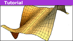
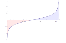
Let us consider an example and define ##f(x,y)=x\cdot |x|\cdot e^{-x^2y^2}.## Therefore
\begin{align*}
\dfrac{d}{dx}\int_\mathbb{R} f(x,y)\,dy&=\dfrac{d}{dx}\int_\mathbb{R}x |x| e^{-x^2y^2}\stackrel{t=xy}{=}\dfrac{d}{dx}x\int_\mathbb{R}e^{-t^2}\,dt=\sqrt{\pi}\\[6pt]
\int_\mathbb{R} \dfrac{\partial }{\partial x}f(x,y)\,dy&=\int_\mathbb{R} \dfrac{\partial }{\partial x}x |x| e^{-x^2y^2}\,dy=2\int_\mathbb{R}\left(|x|e^{-x^2y^2}- |x|x^2y^2 e^{-x^2y^2}\right)\,dy\\[6pt]
&\stackrel{t=xy\, , \,x\neq 0}{=}2 \int_\mathbb{R}e^{-t^2}\,dt -2 \int_\mathbb{R}t^2e^{-t^2}\,dt =2\sqrt{\pi}-2\dfrac{\sqrt{\pi}}{2}=\sqrt{\pi}
\end{align*}

This shows us that differentiation under the integral works fine for ##x\neq 0## whereas at ##x=0## we have
$$
\sqrt{\pi}=\dfrac{d}{dx}\int x\cdot |x|\cdot e^{-x^2y^2}\,dy \neq\int \dfrac{\partial }{\partial x}x\cdot |x|\cdot e^{-x^2y^2}\,dy=0
$$
The missing condition is …

… if ##\mathbf{f(x,y)}## is continuously differentiable along the parameter ##\mathbf{x}.##

Residues

Residue calculus deserves an article on its own, see [7]. So we will only give a few examples here. Residue calculus is the art of solving real integrals (and complex integrals) by using complex functions and various theorems of Augustin-Louis Cauchy.

Let ##f(z)## be an analytic function ##f(z)## with a pole at ##z_0## and
$$f(z)=\sum_{n=-\infty }^\infty a_n (z-z_0)^n\; , \;a_n=\displaystyle{\dfrac{1}{2\pi i} \oint_{\partial D_\rho(z_0)} \dfrac{f(\zeta)}{(\zeta-z_0)^{n+1}}\,d\zeta}$$ be the Laurent series of ##f(z)## on a disc with radius ##\rho## around ##z_0.## The coefficient at ##n=-1## is called the residue of ##f## at ##z_0,##
$$
\operatorname{Res}_{z_0}(f)=a_{-1}=\dfrac{1}{2\pi i} \oint_{\partial D_\rho(z_0)} f(\zeta) \,d\zeta.
$$

Mellin-Transformation.

$$
\int_0^\infty x^{\lambda -1}R(x)\,dx=\dfrac{\pi}{\sin(\lambda \pi)}\sum_{z_k}\operatorname{Res}_{z_k}\left(f\right)\; , \;\lambda \in \mathbb{R}^+\backslash \mathbb{Z}
$$
where ##R(x)=p(x)/q(x)## with ##p(x),q(x)\in \mathbb{R}[x],## ##q(x)\neq 0 \text{ for }x\in \mathbb{R}^+,## ##q(z_k)=0## for poles ##z_k\in \mathbb{C}## and the integral exists, i.e. ##\lambda +\deg p<\deg q.##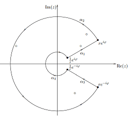Note that
$$
f(z)\,dx:={(-z)}^{\lambda -1}R(z)=\exp\left((\lambda -1)\log(-z)\right)R(z)
$$
is holomorphic for ##z\in \mathbb{C}\backslash \mathbb{R}^+## if we chose the main branch of the complex logarithm. We define a closed curve
$$
\alpha=\begin{cases}
\alpha_1(t)=te^{i\varphi }&\text{ if } t\in \left[1/r,r\right]\\
\alpha_2(t)=re^{it}&\text{ if }t \in\left[\varphi ,2\pi -\varphi \right]\\
\alpha_3(t)=-te^{-i\varphi }&\text{ if }t\in \left[-r,-1/r\right]\\
\alpha_4(t)=\frac{1}{r}e^{i (2\pi-t)}&\text{ if }t\in \left[\varphi ,2\pi – \varphi \right]
\end{cases}
$$
such that the poles are all enclosed by ##\alpha## for large enough ##r## and small enough ##\varphi## and
$$
\int_{\alpha_1}f(z)\,dz+\underbrace{\int_{\alpha_2}f(z)\,dz}_{\stackrel{\varphi \to 0}{\longrightarrow }\,0}+\int_{\alpha_3}f(z)\,dz+\underbrace{\int_{\alpha_4}f(z)\,dz}_{\stackrel{\varphi \to 0}{\longrightarrow }\,0}=2\pi i \sum_{z_k}\operatorname{Res}_{z_k}\left(f\right)
$$
We can show that
\begin{align*}
\displaystyle{\lim_{\varphi \to 0}}&\int_{\alpha_1}f(z)\,dz=-e^{-\lambda \pi i}\int_{1/r}^r t^{\lambda -1}R(t)\,dt \\
\displaystyle{\lim_{\varphi \to 0}}&\int_{\alpha_3}f(z)\,dz=e^{\lambda \pi i}\int_{1/r}^r t^{\lambda -1}R(t)\,dt
\end{align*}
and finally get
$$
2\pi i \sum_{z_k}\operatorname{Res}_{z_k}\left(f\right) =\lim_{r \to \infty}\int_\alpha f(t)\,dt=2 i \sin(\lambda \pi) \int_{-\infty }^\infty t^{\lambda -1}R(t)\,dt.
$$

The sinc Function.

The sinc function is defined as ##\operatorname{sinc}(x)=\dfrac{\sin x}{x}## for ##x\neq 0## and ##\operatorname{sinc(0)=1}.##
\begin{align*}
\int_0^\infty \dfrac{\sin x}{x}\,dx&=\dfrac{1}{2}\lim_{r \to \infty}\int_{-r}^r\dfrac{e^{iz}-e^{-iz}}{2i z}\,dz=\operatorname{Res}_0\left(\dfrac{e^{iz}}{4 i z}\right)=\dfrac{\pi}{2}
\end{align*}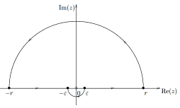

Rules for Residues.

We finally include some general calculation rules for residue calculus that we took from [7].
$$
\begin{array}{ll} \operatorname{Res}_{z_0}(\alpha f+\beta g)=\alpha\operatorname{Res}_{z_0}(f)+\beta\operatorname{Res}_{z_0}(g) &(z_0\in G \, , \,\alpha, \beta \in \mathbb{C}) \\[16pt] \operatorname{Res}_{z_1}\left(\dfrac{h}{f}\right)=\dfrac{h(z_1)}{f'(z_1)}& \operatorname{Res}_{z_1}\left(\dfrac{1}{f}\right)=\dfrac{1}{f'(z_1)}\\[16pt] \operatorname{Res}_{z_m}\left(h\dfrac{f’}{f}\right)=h(z_m)\cdot m&\operatorname{Res}_{z_m}\left(\dfrac{f’}{f}\right)=m\\[16pt] \operatorname{Res}_{p_1}(h\cdot f)=h(p_1)\cdot \operatorname{Res}_{p_1}(f)&\operatorname{Res}_{p_1}(f)=\displaystyle{\lim_{z \to p_1}((z-p_1)f(z))}\\[16pt] \operatorname{Res}_{p_m}(f)=\dfrac{1}{(m-1)!}\displaystyle{\lim_{z \to p_m}\dfrac{\partial^{m-1} }{\partial z^{m-1}}\left( (z-p_m)^m f(z) \right)}&\operatorname{Res}_{p_m}\left(\dfrac{f’}{f}\right)=-m\\[16pt] \operatorname{Res}_{\infty }(f)=\operatorname{Res}_0\left(-\dfrac{1}{z^2}f\left(\dfrac{1}{z}\right)\right)&\operatorname{Res}_{p_m}\left(h\dfrac{f’}{f}\right)=-h(p_m)\cdot m\\[16pt] \operatorname{Res}_{z_0}(h)=0 & \operatorname{Res}_0\left(\dfrac{1}{z}\right)=1\\[16pt] \operatorname{Res}_1\left(\dfrac{z}{z^2-1}\right)=\operatorname{Res}_{-1}\left(\dfrac{z}{z^2-1}\right)=\dfrac{1}{2}&\operatorname{Res}_0\left(\dfrac{e^z}{z^m}\right)=\dfrac{1}{(m-1)!}
\end{array}
$$

Sources