Yardsticks to Metric Tensor Fields
I asked myself why different scientists understand the same thing seemingly differently, especially the concept of a metric tensor. If we ask a topologist, a classical geometer, an algebraist, a differential geometer, and a physicist “What is a metric?” then we get five different answers. I mean it is all about distances, isn’t it? “Yes” is still the answer and all do actually mean the same thing. It is their perspective that is different. This article is supposed to explain how.
The image shows medieval standards of comparison at a church in Regensburg, Germany, Schuh (shoe), Elle (ulna), and Klafter.
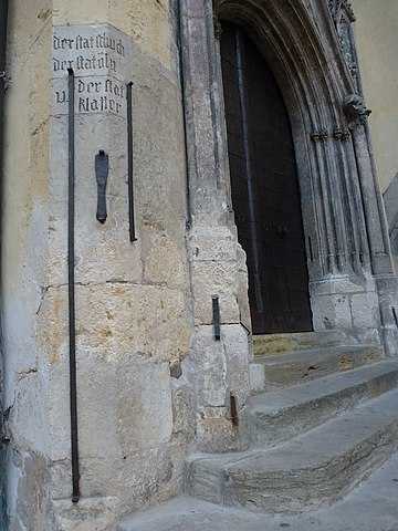
Table of Contents
Topology
The topologist has probably the easiest concept. A metric is a property of certain topological spaces, metric spaces. It means that the topological space is equipped with a yardstick. A function that measures distances. The conditions are clear:
Symmetry
We do not bother whether we measure from right to left or from left to right.
Positive Definiteness
The distance is never negative, and zero if and only if there is no distance between our points, i.e. it is the same point. Sounds silly, but there are indeed exotic topological spaces in which this isn’t a triviality. We just do not want to bother about those pathological examples.
Triangle Inequality
If we are going from one point to another and making a stop at a third point that is not in our direct way, then it is a detour.
Everybody will understand that this is a satisfactory description of what our yardstick is supposed to do.
Classical Geometry
Not so the classical geometer! He does not care about distances. His business is comparisons. No, not shorter or longer. His view is how often one distance fits into another distance. One could argue that this is still the concept of a yardstick: how often does a yard fit into a distance? However, the difference is subtle. The classical geometer does not want to define a unit, be it a yard or a meter. He always compares any two lengths and tells us the quotient of them, e.g. the golden ratio is defined by
$$
\dfrac{a+b}{a}=\dfrac{a}{b}\quad\Longleftrightarrow\quad a^2-b^2=ab.
$$
The ancient Greeks did not only deal with distances. If we look at the trigonometric functions, namely quotients of two lengths again, we get to the other important measure in classical geometry: angles and therewith triangles, preferably right ones. We now have to consider directions, too.
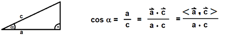
Angles are obviously related to the multiplication of vectors, and that demands two other important conditions, the distributive laws.
Additions
##\langle \vec{a}+\vec{b},\vec{c}\rangle=\langle \vec{a},\vec{c} \rangle +\langle \vec{b},\vec{c} \rangle## and ##\langle \vec{a},\vec{b}+\vec{c} \rangle =\langle \vec{a},\vec{b} \rangle +\langle \vec{a},\vec{c} \rangle##
Stretches and Compressions
i.e. Scalar Multiples
## \alpha \langle \vec{a},\vec{b} \rangle =\langle \alpha \vec{ a},\vec{b} \rangle= \langle \vec{a},\alpha \vec{b} \rangle##
If we now define a length by
$$
\|\vec{a}\| :=\sqrt{\langle \vec{a},\vec{a} \rangle}=\sqrt{\sum_{k=1}^n a_k^2},
$$
we get a metric in the topological sense
$$
d(\vec{a},\vec{b}):=\|\vec{a}-\vec{b}\|=\sqrt{\sum_{k=1}^n (a_k-b_k)^2}.
$$
and an angle
$$
\cos(\sphericalangle(\vec{a},\vec{b}))=\dfrac{\langle \vec{a},\vec{b} \rangle}{\|\vec{a}\|\cdot \|\vec{b}\|}= \dfrac{\sum_{k=1}^na_kb_k}{\sqrt{\sum_{k=1}^n a_k^2}\sqrt{\sum_{k=1}^n b_k^2}}.
$$
Abstract Algebra
An algebraist is interested in the structures, not so much in coordinates, so we define a metric tensor by the properties above rather than coordinates. A metric tensor for a vector space ##V## is therefore simply an element of ##V^*\otimes V^*.## Well, this is true, short, and doesn’t help us at all. What we want to define is an inner product ##\langle \, . \,\, , \,\, . \, \rangle .## That, at its core, is a symmetric, positive definite, bilinear mapping
$$
g\, : \,V \times V \longrightarrow \mathbb{R}
$$
Such a mapping can be written as a matrix ##G,## i.e. ##g(\vec{a},\vec{b})=\vec{a}\cdot G \cdot\vec{b}.## We have considered ##g(\vec{a},\vec{b})=\vec{a}\cdot \operatorname{Id}\cdot\vec{b}## so far, where ##\operatorname{Id}## is the identity matrix. However, there is no reason to restrict ourselves to the identity matrix. Any positive definite matrix ##G## will do. This is basically saying ##g\in V^*\otimes V^*.## Later on, we will even drop this condition and only demand that ##G## is non-degenerate, i.e. that for every vector ##\vec{a}\neq \vec{0}## there is a vector ##\vec{b}## such that ##g(\vec{a},\vec{b})\neq \vec{0}.## With ##G=\operatorname{Id}## we have a specific example of a vector space ##V=\mathbb{R}^n## that gives the construction a meaning.
The metric tensor ##g_p\in V^*\otimes V^*## above an affine point space ##A=\{p\}+V## with translation space ##V## is a mapping that assigns to ##\{p\}## a symmetric, positive definite, bilinear mapping ##g_p.## Length, distance and angle for ##\vec{a},\vec{b}\in V ## are now given as
\begin{align*}
\|\vec{a}\|_p&=\sqrt{g_p(\vec{a},\vec{a})}\\
d_p(\vec{a},\vec{b})&=\|\vec{a}-\vec{b}\|_p\\
\cos(\sphericalangle_p(\vec{a},\vec{b}))&=\dfrac{g_p(\vec{a},\vec{b})}{\|\vec{a}\|_p\cdot\|\vec{b}\|_p}
\end{align*}
If we have an affine linear monomorphism ##\varphi \, : \,\{p\}+U \rightarrowtail \{\varphi(p)\}+V## then any metric tensor on ##\{\varphi(p)\}+V## defines a metric tensor on ##\{p\}+U## by the definition
$$(\varphi^* g)_p(\vec{u}_1,\vec{u}_2):=g_{\varphi(p)}(\varphi_*(\vec{u}_1),\varphi_*(\vec{u}_2)).$$
This pullback, or likewise the fact that ##g_p\in T(V^*),## is the reason the algebraist calls the metric tensor contravariant: Given another monomorphism ##\psi \, : \,\{\varphi(p)\} +V \rightarrowtail \{\psi(\varphi(p))\}+W## then ##(\psi \circ\varphi)^*(g_p)=g_{\varphi(p)}\circ g_{\psi(\varphi(p))}=(\varphi^*\circ \psi^*)(g_p).## This change of order means for mathematicians contravariance. (Attention: physicists call it covariant for different reasons, see below!)
It is important to notice that all three quantities depend on the point ##p.##
Manifolds
All of the above has been rather theoretical so far. Sure, the topologist could explain our yardstick and the ancient Greeks were really excellent in Euclidean geometry. But it is not until we meet the differential geometer and the physicist to tell us something about the real world, the non-Euclidean realities, and the fact that the algebraist’s perspective was not completely irrelevant. They deal e.g. with saddles:
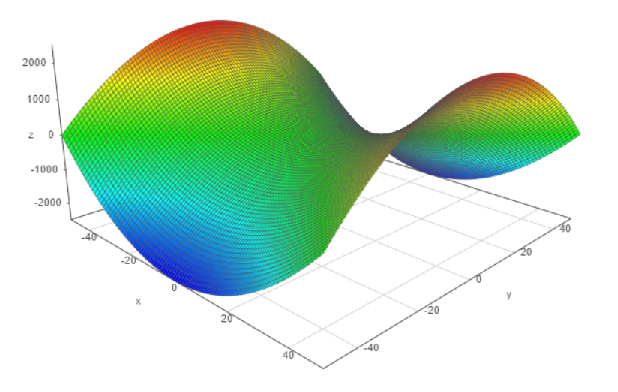
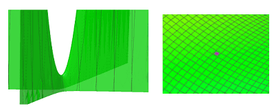
If we increase the resolution, rotate the saddle a bit, and finally zoom in, and concentrate on that small marked square
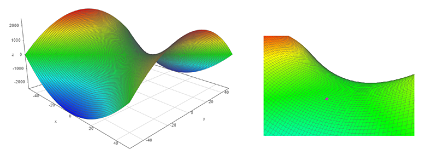
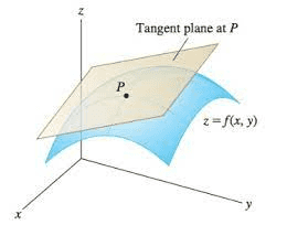
then we can pretend that this is a small flat plane that represents the tangent space at some point within the square. The smaller we choose our square. the smaller the error in any calculations due to curvature. And then we can do the same with any neighboring square. We only demand that the calculations of any overlapping parts have to be the same, for short: charts, an atlas, and an inner product on ##T_pM##.
That’s it. We just have understood the concept of Riemannian manifolds where its local coordinates within the square are the portions of basis tangent vectors of the tangent space at a certain point within the square. Since there is no globally flat coordinate system on the saddle, we have to patch all the tiny flat squares, our charts, and bind them to an atlas. That is what the differential geometer does. Note the big difference between a global view (left) and the local view (right).
One last, but very important note: our manifold here, the saddle, is given by ##M=\{(x,y,x^2-y^2)\,|\,x,y\in \mathbb{R}\}.## This means we have two independent parameters, ##x## and ##y,## so ##\dim M=2,## a surface. And although we have embedded it in our three-dimensional space, we will not care about this embedding, only about the points on ##M.## The only reason for an embedding is, that we can have fancy images. People on earth do not recognize its curvature unless they look at the horizon at sea, big grass savannas, or from outer space.
Physics
Before we listen to the differential geometer who will tell us something about sections and help explain the algebraist, let us hear what the physicist has to say. All of a sudden we find ourselves in a familiar situation.
The affine space is simply ##\{p\}+V=T_pM,## the tangent space at the point ##p## of the manifold ##M## defined by the saddle function ##z=x^2-y^2.## The metric tensor assigns a bilinear form to ##T_pM.## So, depending on where we are, we have length, distance, and angle. But physics is all about measurement. How much differs something if something else happens? In scientific this means: We need coordinates! And since we already understood the Riemannian manifold ##M,## they will be local coordinates; only valid on ##T_pM## and allowing us a reasonable measurement: symmetric, bilinear (distribution laws), and non-degenerate (to allow relativity theory) rather than positive definiteness.
We have seen that it all depends (smoothly) on the location ##p,## which is no surprise since differentiation is a local process. But we can patch all local views to an atlas. This is why we speak of fields instead of spaces. A field is an object obtained by gathering all points ##p\in M.## Therefore we have a metric tensor field, and a tangent vector field. It is usually simply called a vector field, whereas the vector space of tangents is called tangent space.
\begin{align*}
d_p(\vec{x}_1,\vec{x}_2)=\sqrt{g_p(\vec{x}_1-\vec{x}_2,\vec{x}_1-\vec{x}_2)}&\quad\text{ metric}\\
g_p(\vec{x}_1,\vec{x}_2)=D_p\vec{x}_1\otimes D_p\vec{x}_2&\quad\text{ metric tensor}\\
g=\bigsqcup_{p\in M}g_p=\bigcup_{p\in M}\{p\}\times g_p&\quad\text{ metric tensor field}\\
T_pM&\quad\text{ tangent (vector) space}\\
TM=\bigsqcup_{p\in M}T_pM=\bigcup_{p\in M}\{p\}\times T_pM&\quad\text{ (tangent) vector field}
\end{align*}
Coordinates
Let’s consider our saddle ##M=\{(x,y,x^2-y^2):x,y\in \mathbb{R}\}.## A tangent is the velocity vector of a curve ##\gamma :[0,1]\rightarrow M .## We consider ##\gamma^1(t)=(t,p_y,t^2-p_y^2)## and ##\gamma^2(t)=(p_x,t,p_x^2-t^2)## through a point ##p=(p_x,p_y,p_z)\in M## and get the tangents ##\dot\gamma^1(t)=(1,0,2t)## and ##\dot\gamma^2(t)=(0,1,-2t).## They correspond to the vectors fields ##X_1(p)=D_p(x)=(1,0,2p_x)## and ##X_2(p)=D_p(y)=(0,1,-2p_y).##
In terms of level sets, we have ##f(x,y)=x^2-y^2## and ##(p_x,p_y)\in f^{-1}(p_x^2-p_y^2).## Then ##\nabla f(p)=(2p_x,-2p_y).## Let further be ##x,y:[-1,1]\rightarrow f^{-1}(p_x^2-p_y^2)## defined by ##x(t)=(t+p_x,\sqrt{(t+p_x)^2-(p_x^2-p_y^2)}),x(0)=(p_x,p_y)## and ##y(t)=(\sqrt{(t+p_y)^2+(p_x^2-p_y^2)},t+p_y),y(0)=(p_x,p_y).##
Then
\begin{align*}
\nabla(f(x(0)))\cdot \dot x(0)&=(2p_x,-2p_y)\cdot (1,p_x/p_y)=0\\
\nabla(f(x(0)))\cdot \dot y(0)&=(2p_x,-2p_y)\cdot (p_y/p_x,1)=0
\end{align*}
and the tangent space to the level set in ##\mathbb{R}^2## is ##\left\{\nabla f(p)\right\}^\perp = \operatorname{lin}_\mathbb{R}\left\{(p_y,p_x)\right\}##. Thus ##(p_y,p_x,0)=p_yX_1(p)+p_xX_2(p)## is one tangent vector to ##M## at ##p## in the ##z##-plane.
The tangent space with origin in ##p=(2,1,3)## is
$$
T_pM=
\operatorname{lin}_\mathbb{R}\left\{X_1(p)=\left.\dfrac{\partial }{\partial p_x}\right|_p,X_2(p)=\left.\dfrac{\partial }{\partial p_y}\right|_p\right\}=\operatorname{lin_\mathbb{R}}\left\{\begin{pmatrix}1\\0\\4\end{pmatrix},\begin{pmatrix}0\\1\\-2\end{pmatrix} \right\}
$$
and the vector field is
$$
TM = \bigsqcup_{p\in M}\operatorname{lin}_\mathbb{R}\left\{X_1=\dfrac{\partial }{\partial p_x},X_2=\dfrac{\partial }{\partial p_y}\right\}=\bigsqcup_{p\in M}\operatorname{lin}_\mathbb{R}\left\{\begin{pmatrix}1\\0\\2p_x\end{pmatrix},\begin{pmatrix}0\\1\\-2p_y\end{pmatrix} \right\}.
$$
However, we do not want to bother with the embedding in ##\mathbb{R}^3.## The whole idea about manifolds is, that they do not require an embedding. There is no Euclidean space around the universe, only the universe itself. Well, we start a bit smaller and see what the saddle will tell us. But who knows, maybe the universe is a saddle, say a hyperbolic paraboloid. The metric tensor needs vectors as inputs. Our vectors are the tangent vectors ##\{X_1(p),X_2(p)\}## which form a basis for ##V=T_pM.## The affine space ##A## we have spoken about in the algebra section is simply ##A=\{p\}+T_pM.## These spaces are all two-dimensional, so ##g_p## will have four components. In order to illustrate the dependency on location, we define according to the frame ##\mathbf{f}=\{X_1(p),X_2(p)\}##
\begin{align*}
g_p&\triangleq G[\mathbf{f}]=g_{ij}[\mathbf{f}]=\begin{pmatrix}
\cosh^2 p_x +\sinh^2 p_y &0\\0&(1+4p_x^2+4p_y^2)^{-1}
\end{pmatrix}.
\end{align*}
If we change the coordinates in ##T_pM## by
##
U_k=(A_{ij})\cdot X_k=\sum_{l}a_{lk}X_l={a^l}_kX_l
##
then (changing the frame)
\begin{align*}
g(U_i,U_j)&= g({a^k}_i X_k,{a^l}_jX_l)={a^k}_i{a^l}_jg(X_k,X_l)\\
&={a^k}_i{a^l}_jg_{kl}[\mathbf{f}]=\sum_{k,l}(A_{ki})g_{kl}(A_{lj})[\mathbf{f}]=\left(A^\tau \cdot G[\mathbf{f}]\cdot A\right)_{ij}
\end{align*}
and ##G[A\mathbf{f}]=A^\tau G[\mathbf{f}]A,## i.e. the metric tensor, or rather its coordinate representation, is called covariant in physics since its components transform like the basis under a change of coordinates in each index of the frame.
If we change the coordinate functions ##p_x,p_y:M\rightarrow \mathbb{R}## to ##q_x,q_y:M\rightarrow \mathbb{R}## then
$$
\dfrac{\partial }{\partial q_x}=\dfrac{\partial p_x}{\partial q_x}\dfrac{\partial }{\partial p_x}+\dfrac{\partial p_y}{\partial q_x}\dfrac{\partial }{\partial p_y}\; , \;\dfrac{\partial }{\partial q_y}=\dfrac{\partial p_x}{\partial q_y}\dfrac{\partial }{\partial p_x}+\dfrac{\partial p_y}{\partial q_y}\dfrac{\partial }{\partial p_y}
$$
and with the Jacobi matrix ##Dq(p)##
\begin{align*}
g_{q(p)}&=g\left(\dfrac{\partial }{\partial q_x},\dfrac{\partial }{\partial q_y}\right)=g\left(\dfrac{\partial p_x}{\partial q_x}\dfrac{\partial }{\partial p_x}+\dfrac{\partial p_y}{\partial q_x}\dfrac{\partial }{\partial p_y}\, , \,\dfrac{\partial p_x}{\partial q_y}\dfrac{\partial }{\partial p_x}+\dfrac{\partial p_y}{\partial q_y}\dfrac{\partial }{\partial p_y}\right)
\end{align*}
$$
g_{q(p)}=\left(\left(Dq(p)\right)^{-1}\right)^\tau g(p)\left(Dq(p)\right)^{-1}
$$
The tangent vectors in our example are already orthogonal and both diagonal entries are everywhere positive. ##g_p## has therefore the signature ##(+,+)## and is a Riemannian metric.
What is a length according to a metric tensor? The line element can be thought of as a line segment associated with an infinitesimal displacement vector
$$
ds^2=\sum_{i,j}g_{ij}dx_idx_j=g_{ij}dx^idx^j=g_{ij}\dfrac{dx^i}{dt}\dfrac{dx^j}{dt}dt^2 =g[\mathbf{f}]
$$
since it defines the arclength by
$$
s=\int_a^b \sqrt{|ds^2|}=\int_a^b\sqrt{\left|g_{ij}(\gamma(t))\left(\dfrac{d}{dt}x^i \circ \gamma(t)\right)\left(\dfrac{d}{dt}x^j \circ \gamma(t)\right)\right|}\,dt.
$$
The line element completely defines the metric tensor since we considered arbitrary curves. That is why it is often used as a characterization of the metric tensor rather than the actual tensor product. In our example we have (with ##X_1=D_p(x)=dp_x## and ##X_2=D_p(y)=dp_y##)
$$
ds^2=g=(\cosh^2 p_x +\sinh^2 p_y )\,dp_x^2+(1+4p_x^2+4p_y^2)^{-1}\,dp_y^2
$$
The notation of the coordinate functions as ##p_x,p_y## are meant to demonstrate that we are considering real valued functions ##M\to \mathbb{R}.## The usual notation is
$$
ds^2=g=(\cosh^2 x +\sinh^2 y )\,dx^2+(1+4x^2+4y^2)^{-1}\,dy^2.
$$
The metric tensor at ##(0,0,0)## is given as ##g(0,0,0)=ds^2=dx^2+dy^2## and therefore the Euclidean metric. The angle between the two basis vectors is ##\cos\sphericalangle\left( X_1(0,0,0),X_2(0,0,0)\right)=0,## i.e. the basis vectors are orthogonal. At ##p=(2,1,3)## we have a different metric but still an orthogonal basis since ##g(2,1,3)((1,0),(0,1))=0## due to the fact that ##g[\mathbf{f}]## is diagonal and ##[\mathbf{f}]## an orthogonal frame. But the lengths of the basis vectors are no longer ##1.##
\begin{align*}
X_1(2,1,3)&=\|(1,0)\|_{(2,1,3)}=\sqrt{\cosh^2(2)+\sinh^2(1)} \approx 3.94\\
X_2(2,1,3)&=\|(0,1)\|_{(2,1,3)}= \sqrt{1/21}\approx 0.22
\end{align*}
Differential Geometry
The differential geometer and the physicist share the toolbox, but not necessarily the perspective. The main difference might be the degree of abstraction. Emmy Noether spoke of independent variables ##p_x,p_y##, dependent functions ##q_x(p_x,p_y),q_y(p_x,p_y),## and the application of a group of transformations. Modern differential geometers speak of sections and principal fiber bundles, or Euler-Lagrange equations and differential operators. Emmy Noether’s original paper [9] is to some extend easier to understand than the modern treatment of her famous theorem, cp. [11].
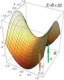
The graph of the function ##f:B\longrightarrow \{z\}## is ##\{(x,y,x^2-y^2)\}=B \times \{z\}=E\cong \mathbb{R}^3.## ##B## is called the base space, here the ##(x,y)##-plane, and ##E## the total space, here the entire ##\mathbb{R}^3.## We have a natural projection ##\pi:E\longrightarrow B\, , \,(x,y,z)\mapsto (x,y).## Any smooth function ##\sigma :B\longrightarrow E## such that ##\pi(\sigma (x,y))=(x,y)## is called a section, and the set of all sections is denoted by ##\Gamma(E).## But what does this have to do with differentiation and the saddle? We already introduced the (tangent) vector field, which is also called tangent bundle or just vector bundle.
$$
E=TM=\bigsqcup_{p\in M}T_pM=\bigcup_{p\in M}\{p\}\times T_pM
$$
where the tangent spaces are the base space isomorphic to ##\mathbb{R}^2## and ##\sigma(p_x,p_y)=(p_x,p_y,p_x^2-p_y^2)## are the sections. The preimage ##\pi^{-1}(p_x,p_y)=\{p\}\times T_pM## is called fiber (over ##p=(p_x,p_y)##). Bundle because we consider sets of points, i.e. bundles (sets) of fibers. This is also the reason why we use the notation with ##\sqcup_p.## To be precise, we should have introduced the cotangent bundle instead because our metric tensor is defined as
$$
\Gamma((TM\otimes TM)^*\ni g \, , \,g_p \in T_p^*M\otimes T_p^*M = (T_pM\otimes T_pM)^*
$$
If we have a group operating on the fibers then we speak of principal bundles. Emmy Noether’s group of smooth transformations is the group that operates on a principle bundle, and its smoothness qualifies it as a Lie group.
Levi-Civita Connection
A connection is a directional derivative in terms of vector fields comparable with the gradient. The Levi-Civita connection is torsion-free and preserves the Riemannian metric tensor. It is also called the covariant derivative along a curve
$$
\nabla_{\dot\gamma(0)} \sigma(p) =(\sigma \circ \gamma )'(0)=\lim_{t \to 0}\dfrac{\sigma (\gamma (t))-\sigma (p)}{t},
$$
or Riemannian connection. Its existence and uniqueness are sometimes called the fundamental theorem of Riemmanian geometry. An (affine) connection is formally defined as a bilinear map
$$
\nabla\, : \,\Gamma(TM)\times\Gamma(TM) \longrightarrow \Gamma(TM)\, , \,(X,Y)\longmapsto \nabla_XY
$$
that is ##C^\infty (M)##-linear in the first argument, ##\mathbb{R}##-linear in the second, and obeys the Leibniz rule ##\nabla_X(h\sigma )=X(h)\cdot \sigma +h\cdot \nabla_X(\sigma).## The Levi-Civita connection is an affine connection that is torsion-free, i.e. ##\nabla_XY-\nabla_YX=[X,Y]## with the Lie bracket of vector fields, and preserves the metric, i.e.
$$
Z(g(X,Y))=g(\nabla_Z X,Y)+g(X,\nabla_Z Y))\text{ or short }\nabla_Z g(X,Y)=0.
$$
The difference to a Lie derivative is, that a Lie derivative is ##\mathbb{R}##-linear but doesn’t have to be ##C^\infty (M)##-linear. We also mention the Koszul formula
\begin{align*}
g(\nabla_{X}Y,Z)&={\tfrac{1}{2}}{\Big \{}X{\bigl (}g(Y,Z){\bigr )}+Y{\bigl (}g(Z,X){\bigr )}-Z{\bigl (}g(X,Y){\bigr )}\\&\phantom{=}+g([X,Y],Z)-g([Y,Z],X)-g([X,Z],Y){\Big \}}.
\end{align*}
If we write with Christoffel symbols ##\Gamma_{ij}^k##
$$
\nabla_j\partial_k =\Gamma_{jk}^l\partial_l
$$
then $$
\nabla_XY=X^j\left(\partial_j(Y^l)+Y^k\Gamma_{jk}^l\partial_l\right) $$
and ##\nabla## is compatible with the metric if and only if
$$\partial_{i}{\bigl (}g(\partial_{j},\partial_{k}){\bigr )}=g(\nabla_{i}\partial_{j},\partial_{k})+g(\partial_{j},\nabla_{i}\partial_{k})=g(\Gamma_{ij}^{l}\partial_{l},\partial_{k})+g(\partial_{j},\Gamma_{ik}^{l}\partial_{l}),$$
i.e. ##\partial_{i}g_{jk}=\Gamma_{ij}^{l}g_{lk}+\Gamma_{ik}^{l}g_{jl}.## It is torsion-free if
$$
\nabla_{i}\partial_{j}-\nabla_{j}\partial_{i}=(\Gamma_{jk}^{l}-\Gamma_{kj}^{l})\partial_{l}=[\partial_{i},\partial_{j}]=0,$$
i.e. ##\Gamma_{jk}^{l}=\Gamma_{kj}^{l}.## We can check by direct calculation that
$$\Gamma_{jk}^{l}={\tfrac{1}{2}}g^{lr}\left(\partial_{k}g_{rj}+\partial_{j}g_{rk}-\partial_{r}g_{jk}\right)$$
where ##g^{lr}## stands for the inverse metric ##(g_{lr})^{-1}.##
Let ##\gamma(t):[-1,1]\longrightarrow M## be a smooth curve on the manifold ##M.## A section ##\sigma \in \Gamma(TM)## along ##\gamma ## is called parallel according to ##\nabla## if
$$\nabla_{\dot\gamma(t)}\sigma (\gamma(t))=0 \text{ for all } t.$$
This means in case of tangent vectors of tangent bundles of a manifold that all tangent vectors are constant with respect to an infinitesimal displacement from ##\gamma(t)## in the direction of ##\dot\gamma(t).## A vector field is called parallel if it is parallel with respect to every curve in the manifold. Let ##t_0,t_1\in [-1,1].## Then there is a unique parallel vector field ##Y:M\rightarrow T_{\gamma(t)}M## along ##\gamma ## for every ##X_p\in T_{\gamma(t_0)}M## such that ##X_p=Y_{\gamma (t_0)}.## The function
$$ P_{\gamma(t_{0}),\gamma(t_{1})}\colon \ T_{\gamma(t_{0})}M\to T_{\gamma(t_{1})}M,\quad X_p\mapsto Y_{\gamma(t_{1})} $$
is called parallel transport. The existence and uniqueness follow from the global version of the Picard-Lindelöf theorem for ordinary linear differential equation systems. We have different inner products at ##t_0## and ##t_1,## and thus different metrics. A parallel transport determines what happens along a path from one tangent space to the other.
We have commuting two-dimensional vector fields in our example of the two-dimensional saddle ##M## because the partial derivatives commute. This means we have ##\nabla_{X_1}X_2=\nabla_{X_2}X_1.## Furthermore, the metric is diagonal, i.e. only stretches and compressions along the coordinate functions. Let
$$
%\gamma: [-1,1] \rightarrow M\, , \,\gamma(t)=(2t+1,t+1/2,3(t+1/2)^2)
\gamma : [-1,1] \rightarrow M\, , \,\gamma(t)=(2t+1,t+1/2)
$$
with ##p=\gamma(-1/2)=(0,0)## and ##q=\gamma(1/2)=(2,1).## We need to solve
$$
\nabla_{(2,1)}\sigma(2t+1,t+1/2)= \lim_{t’ \to t}\dfrac{\sigma(2t’+1,t’+1/2)-\sigma(2t+1,t+1/2)}{t’} =0
$$
which is obviously true for a (smooth) section of ##\Gamma(TM).## The parallel transport is simply given by keeping the components of the vector fields. ##X_p=\alpha X_1(p)+\beta X_2(p)## maps to ##Y_{q}=\alpha X_1(q)+\beta X_2(q).## This means in the three dimensions of the embedding
$$
\begin{pmatrix}\alpha \\\beta \\0 \end{pmatrix}\longmapsto \begin{pmatrix}2t+1\\t+1/2\\3(t+1/2)^2\end{pmatrix}+\begin{pmatrix}\alpha \\\beta \\4\alpha t +2\alpha -2\beta t-\beta \end{pmatrix}.
$$
Sources
[1] E. Chisolm, Geometric Algebra, 2012
https://arxiv.org/pdf/1205.5935.pdf
[2] J.A. Thorpe, Elementary Topics in Differential Geometry (Undergraduate Texts in Mathematics), Springer New York. 1979
https://www.amazon.com/Elementary-Differential-Geometry-Undergraduate-Mathematics/dp/0387903577
[3] What is a Tensor: https://www.physicsforums.com/insights/what-is-a-tensor/
[4] Derivatives: https://www.physicsforums.com/insights/pantheon-derivatives-part-iii
[5] Tensor: https://ncatlab.org/nlab/show/tensor
[6] https://de.wikipedia.org/wiki/Metrischer_Tensor
[7] https://www.geogebra.org/3d
[8] https://academo.org/demos/3d-surface-plotter/
[9] Emmy Noether, Invariante Variationsprobleme
https://gdz.sub.uni-goettingen.de/id/PPN252457811_1918
[10] Connections:
https://www.physicsforums.com/threads/arbitrariness-of-connection-and-arrow-on-sphere.922779/#post-5858045
[11] P. Olver, Applications of Lie Groups to Differential Equations,
Springer, GTM 107, New York 1986
https://www.amazon.com/Applications-Differential-Equations-Graduate-Mathematics/dp/0387950001
[12] https://www.wolframalpha.com/
[13] https://www.physicsforums.com/insights/what-are-tensors-and-why-are-they-used-in-relativity/


Maybe in the section
Reference: https://www.physicsforums.com/insights/yardsticks-to-metric-tensor-fields/#respond
Great Job. You can maybe include a quick mention of Urysohn Metrization Lemma in the Topology section
. Maybe some on Leght Spaces.