Quantum Computing for Beginners

Introduction to Quantum Computing

This introduction to quantum computing is intended for everyone and especially those who have no knowledge of this relatively new technology.

This discussion will be as simple as possible. A quantum computer can process a particular type of information much faster than can a ‘conventional’ computer.

Large companies including Google, Microsoft, IBM, and Intel are spending a lot of money and devoting lots of resources to the development of quantum computers and related software and applications.

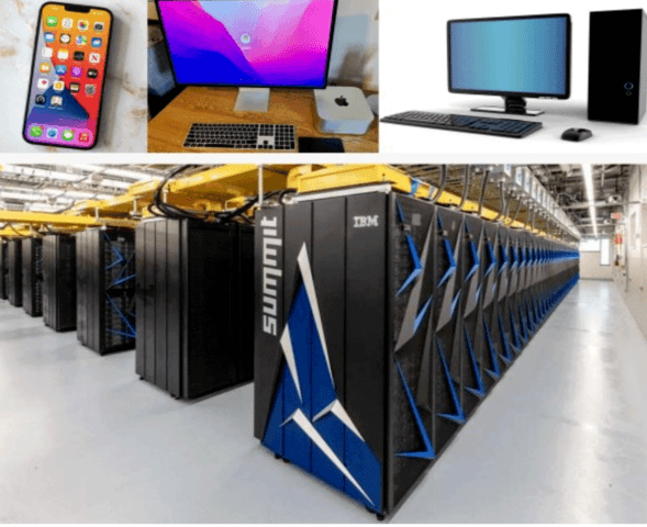
Here are pictures of some conventional computers. They all work the same way in how they process information. The ‘supercomputer’ at the bottom is much faster and more expensive than the others.

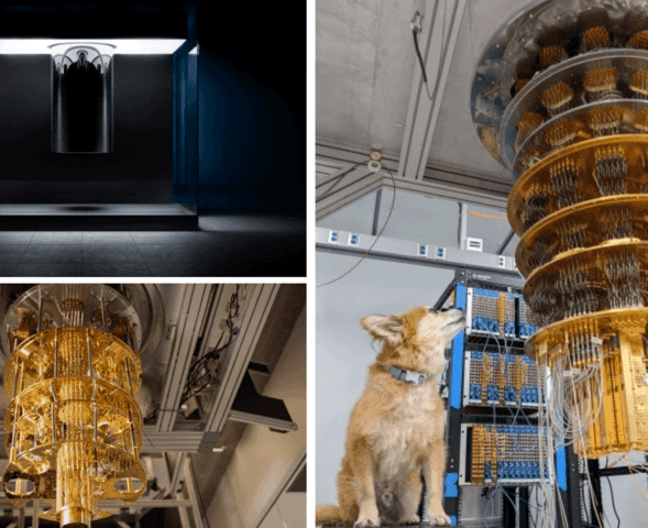
These are quantum computers from IBM, Google, and Microsoft. The dog’s name is Qubit.

Why Quantum Computing?

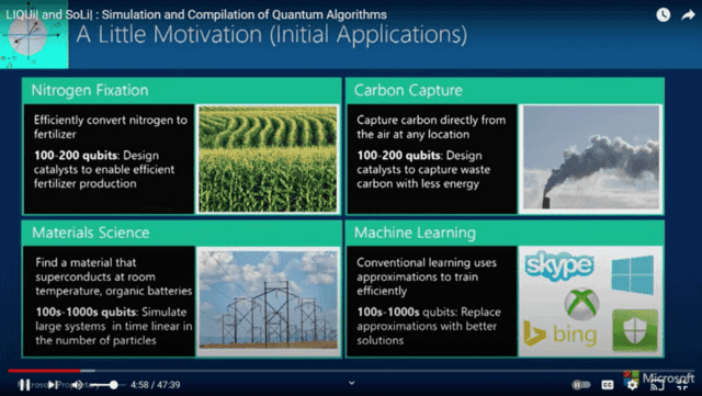
There are certain tasks that cannot be computed by conventional machines because it would take way too long for them to finish.

Creating an efficient way to remove carbon from the atmosphere is a potential Earth-changing application for quantum computers (note 1).

Coins and Information

With a single coin, there are two pieces of information associated with it. The two pieces of information will indicate the coin’s probability of being measured as HEADS or being measured as TAILS.

● We can ‘measure’ the coin by stopping it from spinning and then looking at it, or we can simply look at the coin if it’s not spinning.
● First we are going to place the coin into an initial state. Here this initialized coin will always be equal to HEADS after we measure it.
● For this initialized coin there is a probability of 100% that HEADS will be measured. There is a 0% chance that it will be measured as TAILS. We will write both amounts of probability followed by the resulting states of the coin like this:
● 100/100|HEADS> or 1|HEADS>
● 0/100|TAILS> or 0|TAILS>

● Now we are going to spin the coin. When we measure the spinning coin it will result in the coin being in either the HEADS or the TAILS state with an equal probability.
● Just like the initialized coin there are two pieces of information associated with it. In this case, the two pieces of information are now: 50/100|HEADS> or 1/2|HEADS> 50/100|TAILS> or 1/2|TAILS>
● The spins/measurements will get closer to being 50% HEADS and 50% TAILS the more we spin, measure, and tabulate the results.

It’s time to work with three coins.

● Since there are two pieces of information associated with a single coin, it would seem that there are six pieces of information associated with these three coins. However, there is another way of looking at the information contained in these three coins.
● When considering the coins in combination there are eight pieces of information associated with three coins. These eight pieces of information reflect the probabilities of measuring the three coins in these states:
|HEADS HEADS HEADS>
|HEADS HEADS TAILS>
|HEADS TAILS HEADS>
|HEADS TAILS TAILS>
|TAILS HEADS HEADS>
|TAILS HEADS TAILS>
|TAILS TAILS HEADS>
|TAILS TAILS TAILS>

First, the three coins will be placed into their initialized state.

● When the three coins are measured they will all be HEADS.
● The eight probabilities associated with these three initialized coins are:
1|HEADS HEADS HEADS> All three coins will always measure HEADS
0|HEADS HEADS TAILS>
0|HEADS TAILS HEADS>
0|HEADS TAILS TAILS>
0|TAILS HEADS HEADS>
0|TAILS HEADS TAILS>
0|TAILS TAILS HEADS>
0|TAILS TAILS TAILS>

Let’s put the three coins into their spinning states. Now all eight of the states of the three coins will have equal probabilities of one-out-of-eight.

1/8|HEADS HEADS HEADS>
1/8|HEADS HEADS TAILS>
1/8|HEADS TAILS HEADS>
1/8|HEADS TAILS TAILS>
1/8|TAILS HEADS HEADS>
1/8|TAILS HEADS TAILS>
1/8|TAILS TAILS HEADS>
1/8|TAILS TAILS TAILS>

In general, the number of pieces of information for any given number of coins is: = 2^number_of_coins That is, multiply the number 2 together as many times as you have coins.

Let’s imagine that we have 100 coins.

The number of pieces of information associated with these 100 coins is:
= 2^100 pieces of information for 100 coins
= 2*2*2*2*2*2*2*2*2*2*2*2*2*2*2*2*2*2*2*2*
2*2*2*2*2*2*2*2*2*2*2*2*2*2*2*2*2*2*2*2*
2*2*2*2*2*2*2*2*2*2*2*2*2*2*2*2*2*2*2*2*
2*2*2*2*2*2*2*2*2*2*2*2*2*2*2*2*2*2*2*2*
2*2*2*2*2*2*2*2*2*2*2*2*2*2*2*2*2*2*2*2 pieces of information for 100 coins
= (approximately) 1,000,000,000,000,000,000,000,000,000,000 pieces of information for 100 coins
= one-million-trillion-trillion pieces of information for 100 coins

This is obviously a lot of information.

Quantum Binary Digits (Qubits)

Quantum computers use quantum binary digits or qubits.

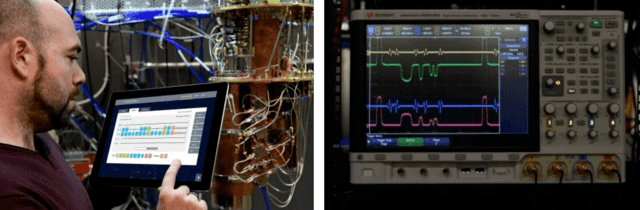
● Qubits are ‘zapped’ by the user in order to modify and then measure their states (note 2). Measuring each qubit reveals one of its two possible values to us.
● These pictures show a quantum computer being programmed, and an oscilloscope display showing the waveforms of the microwave energy that is zapping the qubits.

Qubits and Information

Similar to how we described the operation done on a coin, a qubit when measured will result in it having one of two values.

● Associated with the combinations of qubits are also probabilities regarding what the measured values of the individual qubits might be.
● Each of the possible combinations for the qubits is called a ‘basis state’.
● Unlike coins, however, the amounts of the probabilities for each basis state are progressively modified by the user of a quantum computer. This continues until the user measures the qubits in order to reveal a meaningful answer.

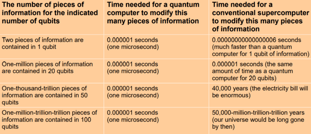
The time required to zap qubits and modify all of their associated basis state probabilities is very fast (note 3).

● On the other hand, if a conventional supercomputer is used to modify similar amounts of probability information it can take a long time.
● This table compares how long it might take a quantum computer and a conventional supercomputer to modify the same amount of probability information (note 4).

Grover’s Algorithm

Here is a simple example of how the algorithm known as Grover’s algorithm might operate on a quantum computer.
● Grover’s algorithm can be used for searching.
● First we are going to consider a Grover’s algorithm that is searching through 16 envelopes (aka basis states).
● 15 of the 16 envelopes each has a worthless small green piece of paper inside.
● 1 of the 16 envelopes contains a one-thousand-dollar bill.
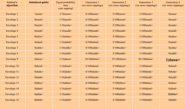
● The algorithm works by successively zapping four qubits in order that the probability associated with one of the sixteen possible basis states becomes much larger than the other fifteen basis states. The basis state with the highest probability is the envelope with the prize.

This table shows how the sixteen basis states of the four qubits change from the initialized state, then to the equal-probability state, and then through four generations of basis state probability updates (note 5).

● The two possible measured states for each qubit will be written as:
|u>
|d>
● The sixteen basis states will range from |uuuu> through |dddd>
● Notice that in Generation 4 the probability amount for one of the sixteen basis states ends up being equal to 1. This is the envelope with the money since all passes through the algorithm and then measurement of the four qubits will always yield the |duuu> basis state.

Shor’s Algorithm

We will conclude with a brief discussion of Shor’s algorithm. It was created by Peter Shor in 1994. Its main feature is that it can factor a very large number much faster when run on a quantum computer than on a conventional computer. Since its creation in 1994, Shor’s algorithm has raised awareness of the potential of quantum computing.

● For the one-digit number ‘6’ it is easy to find its two prime factors.
● For the two-digit number ’15’ it is also very easy to factor.
● The three-digit number ‘143’ might take a fourth-grade student a couple of minutes to find the two factors ’11’ and ’13’.
● A number with six-hundred digits is effectively impossible for classical supercomputers to factor because it would take them trillions of years to find the two factors.
● The RSA and Diffie-Hellman encryption schemes are what keep our internet transactions secure because they utilize a technique that requires the factoring of a six-hundred digit number (2048 bits) in order to break the encryption.
● A large enough quantum computer (6,000 error-corrected qubits) will be able to factor a six-hundred digit number in less than an hour.
● We are many years away from having a quantum computer large enough to threaten our online data security. There are also quantum encryption schemes being developed that will keep us safe. Quantum encryption is way ahead of classical encryption breaking.

Notes And Other Resources

Link to a video discussing carbon capture (at 3min50s) – https://www.youtube.com/watch?v=4mMizLpIVKs

‘Zapping’ and ‘measuring’ certain types of qubits involves exposing the qubits to precise amounts of
microwave electromagnetic radiation.

Zapping a single qubit or even multiple qubits will probably be around one microsecond. For small quantum
computers this is currently faster, but when large amounts of qubits become available then multiplexing and
demultiplexing of the zapping waveforms will likely be used.

To simulate changing the state of entangled qubits by a conventional computer, the current 2^n length state
vector of the qubits is multiplied by a 2^n by 2^n square matrix. This requires 2^2n multiply/add operations by
the conventional computer. The supercomputer speed used in the time calculations is one-exaflops (10^18
floating point operations per second).

The specific Grover’s algorithm used in the simulation for the values shown in the table is from Fig.1d here:
https://www.nature.com/articles/s41467-017-01904-7

Other resources:
The Sounds of IBM – IBM: https://www.youtube.com/watch?v=o-FyH2A7Ed0
Inside the Google Quantum AI Campus – Google: https://www.youtube.com/watch?v=2uV5XwhH6Eg
The Map of Quantum Computing – Domain of Science: https://www.youtube.com/watch?v=-UlxHPIEVqA