Approximate LCDM Expansion in Simplified Math (Part 2)
Table of Contents
Part 2: Time and Distance
In Part 1 we have seen how one of the simplest ways of expressing the fractional expansion rate of the universe, i.e. the Hubble value H, is with this equation:
2.1 [itex]H = (0.44 S^3+1)^{0.5}[/itex] zeit-1
Here S is the ‘stretch factor’, which is the inverse of the scale factor a, i.e. S=1/a. By convention, S have a present value of 1.0; hence the present Hubble value H0 = (1.44)0.5 = 1.2 zeit-1. But what is the relationship between H and cosmological time?
Cosmological Time
Because of the instantaneous “interest on interest” nature of cosmic expansion, it follows an exponential pattern (eHt), provided that H remains constant over time. Presently H is still decreasing, so cosmological time is approximated by the following natural logarithmic equation:[1]
(2.2) [itex]\large t = \frac{1}{3}\ln(\frac{H+1}{H-1})[/itex] zeit.
Let us put our present H0 = 1.2 zeit-1 in here (using Google or some other calculator) and check that we get the 0.8 zeit that we expect.
[itex]t_{now} = \frac{1}{3}\ln(\frac{2.2}{0.2})\approx 0.8[/itex] zeit.
Suppose we observe the redshift from a specific galaxy as z=1, which means that the light has left it when the wavelength stretch factor was S = z+1 = 2. Plugging S = 2 into eq. 2.1, we find that H = 2.13 zeit-1 when the light was emitted. The cosmic time was
[itex]t_{then} = \frac{1}{3}\ln(\frac{2.13+1}{2.13-1})\ = 0.34[/itex] zeit after the start of the present expansion.[2]
The light from that galaxy obviously took 0.8 – 0.34 = 0.46 zeit to reach us – it is the so-called ‘lookback time’.
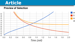
Now that we have a feeling for the relationships, what is better than viewing it on a graph? Here you see the parameters mentioned so far (against time).
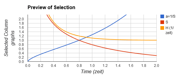
Fig: 2.1: Scale factor (a) , Stretch factor (S) and Hubble value (H) against time
You can see our present time (0.8 zeit) clearly where the red and blue curves cross, i.e. where both S and a are unity. You can also see how H starts high and asymptotically approaches unity. The graphs were plotted using LightCone 7zeit, a variant of the standard LightCone 7.
I have ‘sneaked in’ the curve for the scale factor (a=1/S), but I did not give a direct relationship of it against time yet. You get it by solving eqs. 2.1 and 2.2 simultaneously, which is not a simple exercise at all. Fortunately, mathematics comes to the rescue and we have a nifty solution for a(t), i.e. the scale factor as a function of time:
(2.3) [itex]\Large a(t) = \frac{\sinh^{2/3}(\frac{3}{2}t)}{1.3} [/itex]
where sinh is the hyperbolic sine function. The ‘hypersine’ is obviously related to the natural logarithm ln(x) and the natural exponent (ex). The factor 1.3 is just scaling to make anow = 1 at tnow = 0.8 zeit, as is the convention. The importance of a(t) is that its curve shows how a decelerating expansion gradually changed over to an accelerating expansion. The inflection point can be visually judged to lie between 0.4 and 0.5 zeit. It is actually at 0.44 zeit.
Proper Distance
Proper distance in cosmology is like measuring distance on a hypothetical frozen view of the cosmos, i.e. with expansion stopped. Obviously, we cannot stop expansion, so how do we find proper distance? There are various methods, but once we have the present and long-term Hubble values (H0 and H∞), we only need to measure the redshift of a source and then calculate its proper distance from where we are.
Because of the non-linear expansion, there is no precise analytical solution for the proper distance (that I know of). We have to numerically integrate into small steps, but fortunately the definite integral is rather neat:
(2.4) [itex]\large D_{now} = \int_1^S{\frac{dS}{H}} = \int_1^S{\frac{ds}{\sqrt{0.44S^3+1}}}[/itex]
We have substituted H from eq. 2.1 in here, so that we have a distance in terms of the observable S = z+1. For calculation, you can use your favorite integrator, but a rather cool web-based one is available at
http://www.numberempire.com/definiteintegralcalculator.php.
For our previous sample galaxy at S=2, I entered 1/sqrt(0.443x^3+1) into the Function box, with 1 in the “From” and 2 in the “To” boxes and then clicked “Compute” – it returned the answer as 0.64, which in our cas has the units lightzeit. So we receive the light when the proper distance to the galaxy is Dnow = 0.64 lzeit. Since we have used stretch S = 2, the proper distance when the photons left the galaxy was half of 0.64, i.e. 0.32 lzeit; so we say that Dthen = 0.32 lzeit for this galaxy. Recall that the light left that galaxy at t = 0.34 zeit, i.e. 0.46 zeit ago. Here is a graph of Dnow and Dthen.
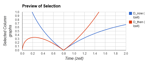
Fig. 2.2: Present proper distance (D_now, also called the comoving distance) and the proper distance when light was emitted, or will be received (D_then, also called the past and future lightcones).
The red Dthen curve is also known as the cosmological lightcone. To the left of 0.8 zeit it represents our past lightcone and to the right of 0.8 zeit our future lightcone. Near t = 0.0 the universe was very dense and objects we now observe were actually very, very close to our space locality. Distances then grew much faster than the progress that photons could make in our direction and ancient photons were at first dragged away from us. At around t = 0.23 zeit, the fractional expansion rate dropped enough to allow photons to make progress and eventually reach our telescopes.
To summarize, we have now looked at a further three rather easy equations that allow us to calculate the most common values for the standard cosmological model.
Part 3 will deal with the Hubble radius and two cosmological horizons that we should take notice of.
End-notes
[1] The function eHt gives the factor by which cosmic distances increase in a time interval t, provided that H remains constant over this time interval. In the far future, H will be a constant, but in the early universe H changed significantly over periods longer than a million years. Hence the more complex general solution.
[2] To verify that the approximations are valid, I used the LightCone 7zeit calculator for a ‘one-shot’ calculation with Supper=2 and Sstep=0.
[3] The Dthen lightcone is where the LightCone 7 calculator got its name from.
Male aerospace engineer
Play music, Read relativity and cosmology


[QUOTE=”Jorrie, post: 5180861, member: 46478″]…
I think the idea of showing some of the other relationships in end-notes is good (or perhaps in an extra appendix).[/QUOTE]
Good. I could contribute a postscript of some sort. I don’t want to intrude on your main text article. It wouldn’t need to be attached.
I see the point of basing the main development on observable quantities, like S. Time is intuitive but elusive. But that would be an easy afterword-type thing for me to write—if you want—the two horizon integrals dt instead of ds.
[QUOTE=”marcus, post: 5180795, member: 66″]
As a comment or addendum it is also possible (though certainly not essential) at that point to give an alternative form of the distance integral with t as the variable and S(t) as the integrand.
[/QUOTE]
Yes, time is a very intuitive variable for us humans, but unfortunately it is not one of the observables in cosmology. The time values we use are very model and parameter dependent. Time against S can also be obtained by a simple integration, similar to the ones discussed here. I am trying to give all derived quantities in terms of the observable (S, z, a and H[SUB]0[/SUB]) in as simple as possible a fashion.
I think the idea of showing some of the other relationships in end-notes is good (or perhaps in an extra appendix).
[QUOTE=”marcus, post: 5180768, member: 66″]
So I cannot comment in the regular Insights comment section. And in this thread we cannot see the original part 2, so I cannot use the REPLY function to obtain copies of equations 2.3 and 2.4. this means my comment is likely to be obscure because it won’t be clear what I am talking about.[/QUOTE]
Yea, there is a bit of ‘disconnect’ (incompatibility) between the Insights system and the normal PF editor. It is also difficult to copy and paste from PF into Insights, but there are workarounds.
You can copy and paste text and equations, but the equations are converted to plain text. I use the windows right-click function on the original equation to show the equation as Tex commands, which can then be copied either way. One need to put the ‘tex’ or ‘itex’ tags in by hand. Cumbersome, but workable.
Basically equation 2.3 introduces the scale factor as a function of the “time then”, t, namely S(t) = 1.3/sinh[SUP]2/3[/SUP](1.5t).
And equation 2.4 gives you the distance integral with S as the variable and H(S) in the denominator.
As a comment or addendum it is also possible (though certainly not essential) at that point to give an alternative form of the distance integral with t as the variable and S(t) as the integrand. IOW cdt is the little step the light takes at time t, and S(t) is the factor by which that step is blown up or shrunk down between time t and the present. So the distance integral is the sum of little steps, each of which has been adjusted for expansion.
The two horizons become$$int_.00001^.8 S(t) dt$$ $$int_.8^infty S(t) dt$$and the transition to the equation 2.4 form of the distance integral is a somewhat messy (but at least not mysterious) change of variable. The actual change-of-variable process is either footnote material or IMHO something hairy to be politely ignored. : ^)
There’s something slightly awkward about the Insights format.
Now that part 3 is posted at Insights, I would like to comment about two equations in part 2, namely equations 2.3 and 2.4. But Insights does not seem to have LaTex.
So I cannot comment in the regular Insights comment section. And in this thread we cannot see the original part 2, so I cannot use the REPLY function to obtain copies of equations 2.3 and 2.4. this means my comment is likely to be obscure because it won’t be clear what I am talking about.
Good. I’ll wait on horizons. Let me know if I should erase any spoilers or edit any of my posts here (intended to explore possible examples and supplemental stuff).
[QUOTE=”marcus, post: 5178455, member: 66″]Explain why this gives, as of today, the distance to the farthest galaxy we could reach with a signal sent today
[tex]int_0^1 ((s/1.3)^3 + 1)^{-1/2}ds[/tex]
[/QUOTE]
You are running ahead of Insights Part 3 now. :wink:
It may be good to make readers think about the horizons in advance, but they are quite tricky to comprehend and I am still working on the best way to present them in concise form.
Is there any merit to getting “transdisciplinary” about this and mixing some biohistory in with our cosmology?
Does it do anything for you to be told that the galaxy disk formed at t=0.29 and Earth formed at expansion age t=0.54 zeit
and that the first evidence of microbial life on Earth dates from t=0.59?
Or that our ancestors the fish did not appear until t=0.77, and even then they did not have [B]jaws[/B]—had not even figured out how to have jaws!
As far as I’m concerned it’s helpful because it helps me get an idea of the passage of time in cosmology to picture the passage of time in other developments like evolution.
Anybody, please tell me if you think these exercise problems are too hard, or don’t belong here. We can always make examples and exercises easier, or eliminate them altogether. But we won’t know if they belong here and are the right compatible level if we don’t try. Here’s one
Explain why this gives, as of today, the distance to the farthest galaxy we could reach with a signal sent today
$$ int_0^1 ((s/1.3)^3 + 1)^{-1/2}ds$$
and explain why this other integral gives, again in terms of today’s distance, the radius of the currently observable universe
$$ int_1^infty ((s/1.3)^3 + 1)^{-1/2}ds$$
that is the current distance to the farthest matter that can have emitted a signal which is arriving now.
What represents the present era, the “now”, in these integrals? How would you change them so as to give the same quantities but for people in the past or future—the radius of observable for some people in the past—the farthest now reachable (cosmic event horizon) for some people in the future, etc.
these integrals are really easy to do at numberempire.com, it even remembers the integrand ((s/1.3)^3 + 1)^{-1/2} so you don’t have to type it in each time. all you do is put in different limits and press calculate.
==============proceed at your own risk================
“For extra credit” what does this signify?$$ int_0^infty ((s/1.3)^3 + 1)^{-1/2}ds$$spoiler: the distance [B]now[/B] to the farthest matter that will EVER be part of our observable. IOW the ultimate max of the “particle horizon” in what is called “comoving distance” ( jargon terms, professional technical vocabulary are often unhelpful, this might be a case of unhelpful jargon, but the idea of permanently assigning to each patch of matter a number which is its distance from us as of today turns out to be very handy)
Later that night you measured the spectrum of light from a different galaxy and found the stretch of that light was S = 1.65.
Think about the situation back when that light was emitted—the distance from that galaxy to the matter that eventually became us, the Earth as we know it, the stuff around us etc.—that distance was expanding, obviously, but was its speed of expansion slowing or speeding up?
Is this exercise too hard? Can someone suggest some more congenial, perhaps easier examples.
The thing is, if you know S then we have formulas for H(S) and D(S) in Jorrie’s treatment (if not in part 2 in part 3) and v=HD
so we have a handle on the speed of that distance’s expansion. “was its speed of expansion slowing or speeding up?” maybe the answer is simply “no”.
: ^)
Still not sure if this kind of supplemental material is sufficiently on-topic. I collected some such “cosmology enrichment” stuff in the “hypersine” thread starting around post #39
[URL]https://www.physicsforums.com/threads/the-hypersine-cosmic-model.819954/page-2#post-5155318[/URL]
Imagine you are an astronomer observing some patch of sky last night and some light comes in with stretch S=2.6
Imagine that light when it was just emitted by its home galaxy. Obviously the light is aimed in our direction because it eventually got here.
Try to picture the situation.
When it was first emitted what kind of progress towards us was it making?
Was it approaching us or was it being swept back by expansion?
At what speed was the distance of the home galaxy from us increasing?
This could be seen as slightly off topic. I’m trying to think of ways to [B]supplement[/B] Jorrie’s treatment of the basic math of standard cosmic model. The treatment is concise and clear. How could we ADD stuff (like examples, exercises, graphics…) to make it more concrete.
For example in the A2z2Z thread [B]Wabbit[/B] posted this:
[QUOTE=”wabbit, post: 5121570, member: 541738″]
==quote==
…because the redshift+1 of the CMB is estimated at 1090, the temperature of the hot gas at last scattering, that emitted the ancient background light, was 2.725*1090 ≈ 3000 kelvin
==endquote==
A pale orange hue then :
[IMG]http://www.techmind.org/colour/blackbodyglowinfinity.png[/IMG]
Unfortunately the current color is off-the chart, in the radio spectrum, so we cannot compare : ([/QUOTE]
[URL]https://www.physicsforums.com/threads/from-aeon-to-zeon-to-zeit-simplifying-the-standard-cosmic-model.811718/page-4#post-5121570[/URL]
It makes it possible for a newcomer to imagine the original CMB light, on the day it stopped getting scattered and got loose to run freely—and it impresses the idea that expansion cools heat-glow light in proportion as it lengthens the wavelengths. this may or may not be worth adding as a footnote somewhere.
Or maybe not even adding, just having a link to it handy as a teaching resource. Wabbit may have other ideas as well.
If it is not too much clutter—or too off-topic—I will try to think up some supplemental material. I like examples that make cosmology more [B]concrete.[/B]
I have to say, Ryan, that I actually [I]learned[/I] quite a bit by trying to answer all your questions occasioned by Part 1 of Jorrie’s Insights article. (We took those questions over to a Cosmology forum thread, A2z2Z, instead of the regular Insights comments section.)
I really must say that struggling with your persistent questions brought me some new understanding of the approach to basic cosmology that Jorrie and I have been working on. It’s good to have someone around with that much curiosity and drive.
I’m looking forward to seeing Jorrie’s [B]Part 3[/B], and hope it will be posted soon.
Great work :)This time I dont have any questions,Thanks Marcus