Approximate LCDM Expansion in Simplified Math (Part 4)
Table of Contents
Part 4: Cosmic Recession Rates
An astronomer, accompanied by his amateur relativist friend, aimed a telescope at a distant galaxy and measured its redshift. It came out at exactly z=2. The astronomer thought for a moment and then said: “The recession rate of this galaxy exceeds the speed of light by about 20%”.
His friend frowned, took out his tablet, tapped around a little, and replied: “Well, not according to Einstein’s Special Relativity. A Doppler redshift of 2 implies a recession speed of 0.8c. And it can never exceed c”.[1]
The astronomer smiled and replied: “My friend, you are right for Minkowski spacetime, but in the long-range astronomy we are working with here, it is not Minkowski spacetime and any recession rate is possible.”
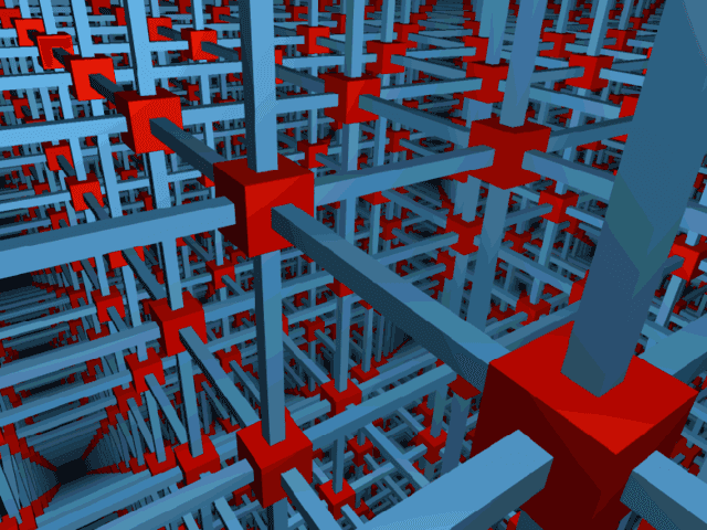
Fig. 4.1 Escher’s Infinite Lattice. Art by Coburt
To better understand why the astronomer was saying this, consider the depiction of ‘Escher’s Infinite Lattice’ in Fig. 4.1. Suppose there are a zillion identical, straight blue bars supporting a zillion red cubes. Also suppose that due to some mechanism, each blue bar is continuously lengthening at a rate of one ‘red cube side length’ per year, while all the cubes remain unaffected, size-wise.
If the lattice is observed ‘from the outside’, against a flat, static background spacetime, then the relativist is right – no cube can recede from any other cube at a rate exceeding ‘c’. However, if the lattice is observed from within, using ‘our cube’s time’ and ‘our cube’s side’ as a standard ruler, then the growth rate is not limited to c. A zillion bars, each lengthening by one cube side per year, will cause an overall lengthening of a zillion cube sides per year.
Another way of looking at it is that cosmological recession rates are quite like the growth rate of money in an investment, which we normally express as a percentage return over a period of time. But, we can also express it as so many dollars earned per time period, which is essentially the present ‘speed of growth’ of the investment. Cosmic recession rates are similar to this sort of speed.
The proper distance of a galaxy is equivalent to the investment amount, the Hubble constant is equivalent to the interest rate and the increase in proper distance is equivalent to the dollars earned. Divide the increase in proper distance (say km) by a time period (say seconds) and you have a recession rate in km/s. The larger the proper distance, the larger the recession rate, without any upper limit.
Present Recession Rate
From the above, it is reasonable to view the present recession rate (Vnow) of a source as
4.1: [itex]\large \frac{V_{now}}{c} = H_{now} D_{now}[/itex]
We had the equations for Hnow and Dnow in terms of the stretch factor (S=z+1) before and we have already calculated the present value of Hnow as 1.2 zeit-1. Hence, from eq. 3.4 in Part 2 we have:
4.2: [itex]\large \frac{V_{now}}{c}= 1.2 \int_1^S{\frac{dS}{\sqrt{0.44S^3+1}}}[/itex]
It gives a dimensionless value, but it is the custom to put the ‘c’ on the other side, i.e. to express the recession rate in units of ‘c’. In the units that we use here (lzeit and zeit), c=1 anyway, so it makes no numerical difference. Here is what the present recession rate looks like against the expansion factor (a=1/S). Time is also shown for convenience.[2]
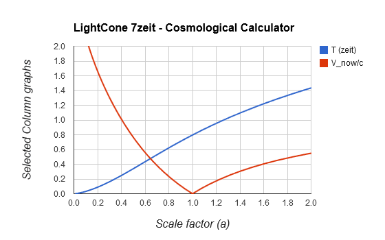
Fig. 4.2 The present recession rate of an observed source that emitted the signal when the scale factor was ‘a’ (for a smaller than 1), or the present recession rate of an observer that will see our present signals in the future, when the scale factor ‘a’ is greater than 1.
For simplicity, we will first discuss only recession rates as observed today (a<1). For a>1 we need to consider observations to be done in the future, which will be dealt with later on in this article. It is clear that for scale factors smaller than around 0.4, the present recession rate is higher than c. This scale factor corresponds roughly with the Hubble radius that we discussed in Parts 2 and 3.
Using eq. 4.2, let us calculate Vnow for our astronomer’s galaxy at redshift z=2 (or stretch S=z+1=3). We enter 1/sqrt(1+0.44*x^3) into the definite integrator, with integration limits set to 1 (now) and 3 (then). It gives back a result: Dnow(S=3) = 1.0 lzeit. We know that our present Hubble value is 1.2 zeit-1, giving Vnow(S=3) = 1.0 x 1.2 = 1.2 c. This means that the proper distance of the observed galaxy presently grows by 1.2 lzeits per zeit, or more conventionally, by 1.2 ly per year.
Past Recession Rate
When the light that we observe today at stretch S has left the galaxy, it was a lot closer and the expansion rate was a lot higher. The recession rate then (Vthen) is simply the Hubble value at the time that the observed light was emitted, multiplied by the proper distance of that galaxy when the observed light was emitted, i.e.
4.3: [itex]\large \frac{V_{then}}{c} = H_{then} D_{then} = H_{then} \frac{D_{now}}{S}[/itex]
We have seen both of these values before. Again using our astronomer’s S=3 galaxy, we can easily determine that the Hubble value when the light has left that galaxy with Google: Hthen = sqrt(0.443*3^3+1)=3.6 zeit-1. The past proper distance Dthen is simply the Dnow that we have determined above (value 1), divided by the stretch factor (S=3). This gives Vthen=3.6 c/3 = 1.2c. Amazingly, this is the same value that we have calculated for Vnow, as if this galaxy has always been receding at 1.2c. This cannot be, as we shall soon discover, but first, here is the ‘now’ and ‘then’ recession rates compared to each other for different values of expansion factor.
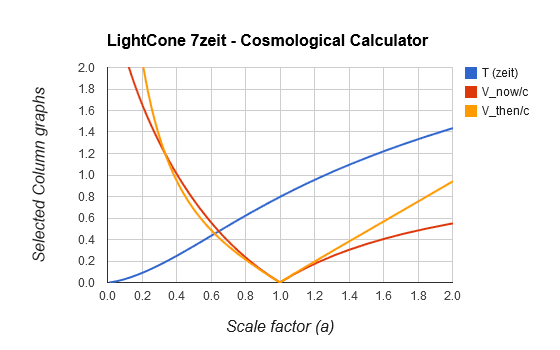
Fig. 4.3 Past recession rate (V_then, gold) of a source that emitted light when scale factor was ‘a’ in comparison to the present recession rate (V_now, red) of the same source.
The past recession curves (i.e. for a<1) must be interpreted as follows: the red curve gives the present recession rate of a galaxy for which the observed light has left it when the scale factor was ‘a’. The gold curve gives the past recession rate of that galaxy. We can easily see that the ‘then’ and ‘now’ recession rates are not generally the same. They just happen to cross when a=0.33 and again today.
Future Recession Rate
The interpretation of the part of the curves to the right of a=1 (i.e. for a>1) is slightly different, because it represents signals that will be received in the future, not by us, but by some distant observer. We send a signal today (a=1) and some observer receives it when the scale factor is greater than 1. Vnow is the present recession rate of that observer and Vthen is the recession rate of that observer when our signal is received.
Let us examine this by means of an example. If we go to the right-hand limits of the Fig. 4.3 and we ask: if we send a signal out today, what will the recession rate of an observer be if it receives our signal when a=2. We can use eq. 4.3, but by simply looking at the gold curve in Fig. 4.3, it is somewhere between 0.9c and 1.0c (it is actually Vthen = 0.94c). The red curve shows that the present recession rate of that observer is around Vnow = 0.55c.
It is not shown in Fig. 4.3, but both future curves will eventually exceed c. Vnow will eventually approach and be limited to 1.144c, but Vthen can increase without limit.[4] What this says is that if the present recession rate of a galaxy is larger than 1.144c, we can no longer communicate with it, even given infinite time. It simply means it is already beyond our communications horizon. We have discussed this horizon in Part 3.
Generic Recession Rate
Up to now we were graphing for different galaxies that are observed at different S values. It is interesting to see how the recession rate of one specific galaxy changes over time, but we need to do a different calculation than before. A generic recession rate (Vgen) can be determined over time by using any galaxy that is presently exactly on the Hubble sphere, i.e. with a present recession rate of exactly ‘c’.[5]
Through some easy algebra, it can be shown that the generic recession rate is simply the ratio between the past and the present recession rates of this ‘generic galaxy’, i.e.[5]
4.4: [itex]\large \frac{V_{gen}}{c} = \frac{V_{then}}{V_{now}}[/itex]
as is shown in the red curve below, together with some previous curves for comparison. Cosmological time is again shown to confirm that the minimum generic recession rate happens at the inflection point, where decelerating expansion goes over into accelerating expansion.[6]
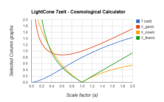
Fig. 4.4 The generic expansion rate (red) against the expansion factor. It is easy to see that V_gen follows the ratio between the green and gold curves (V_then/V_now).
The generic galaxy (presently at a proper distance equal to our Hubble radius) has originally been outside the (increasing) Hubble radius (not shown in Fig. 4.4). Then at a ~ 0.33 (T~ 0.19 zeit) the Hubble radius caught up with the galaxy and its recession rate dropped to below c. After that the generic galaxy lagged farther behind the Hubble radius’ growth for some time. At the inflection point, where accelerated expansion began (a~0.6, T~0.44 zeit), the generic galaxy started to catch up with the Hubble radius again and it is presently (a=1, T~0.8 zeit) crossing it, with the recession rate equal to c once more.
This is part of the reason why we can observe that galaxy at S=3 (and even for much higher values), even though the recession rates now and then were higher than c. At some stage in the past, due to decelerated expansion, the Hubble radius caught up with the galaxy and its recession rate dropped to below c. The main reason is however that the Hubble radius caught up with the photons that were coming our way from even before that time. Those photons could then make headway in our direction (against the ‘weaker current’, so to speak). We have discussed this in Part 2 where we have compared the Hubble radius to our past light cone.
Final Remarks
This ends our little tour through the simplest forms of the basic equations of the LCDM cosmological model. Nothing ground-breaking, just an effort to demystify some of the common values that are written about in the literature. And a relatively easy set of equations for calculating those values, if that is of interest to you.
There are probably many more interesting insights that can be obtained and I invite others to either ask questions or to post some insights that are related to these equations and their graphical presentations. A good place to post (and seemingly with more functionality than in the ‘quick remarks’ portion of the Insights forum) is in the Cosmology section of PF, where a ‘comments’ thread is generated for these Insights posts.
If calculating the values is not your thing, there are many cosmological calculators on the Web, with one particular version customized to this ‘zeit-based’ view of the cosmos. It also includes the early radiation-dominated era and hence some of its results will differ slightly from the simplified equations in these articles.
Endnotes
[1] The special relativistic calculation of relative speed from Doppler shift is:
4.5: [itex]\large v = \frac{(z+1)^2-1}{(z+1)^2+1} c = \frac{S^2-1}{S^2+1} c [/itex]
where we used our customary stretch factor S=z+1 in the second part.
[2] We are usually not plotting against S, because its ascending values point back into the past, hence the graph is not intuitive. The ascending scale factor a=1/S graph ‘runs in the same direction’ as time. Here the scale factor as the independent variable actually gives a more intuitive meaning to the recession rates than what time does.
[3] We could have used any other large distance, but the Hubble radius is a characteristic distance for our universe, where recession rate equals the universal constant ‘c’. For any galaxy, its recession rate curve can be scaled proportionally to its present proper distance as a multiple or fraction of the Hubble radius (0.83 lzeit).
[4] To get the limiting value of the present recession rate, we consider ‘a’ going to infinity, i.e. S approaching zero and H approaching 1 and plug them into the Vnow equation. Since Vthen has a division by S, it means it means it can increase without limit.
[5] The recession rate of a ‘generic galaxy’ (which is presently at the Hubble radius) changes proportionally to the scale factor and the ratio H/H0, so that
4.6: [itex]\large \frac{V_{gen}}{c} = \frac{a H_{then}}{H_{now}} = \frac {aH_{then} D_{now}}{H_{now} D_{now}} = \frac {H_{then} D_{then}}{H_{now} D_{now}} = \frac{V_{then}}{V_{now}}[/itex]
[6] The inflection point is where the time against scale factor curve changes from concave to convex, or convex to concave, depending on from which axis you are viewing.
Male aerospace engineer
Play music, Read relativity and cosmology


[QUOTE=”marcus, post: 5196859, member: 66″]
But how to explain that the expansion age is 0.8 zeit?
It could be that I’m asking how to make it intuitive that we can add a third curve (time) to the graph, just reaching 0.8 at the right edge where a = 1.0.
[URL]https://www.physicsforums.com/insights/approximate-lcdm-expansion-simplified-math-part-4/[/URL][/QUOTE]
I think Fig. 2.2 ([URL]https://www.physicsforums.com/insights/approximate-lcdm-expansion-simplified-math-part-2/[/URL]) is the best to show the 0.8 zeit present time.
[IMG]https://physicsforums-bernhardtmediall.netdna-ssl.com/insights/wp-content/uploads/2015/07/D_now-D_then-vs-t.png[/IMG]
But more curves can be added, as long as it does not interrupt the flow of the Insight posts too much. Perhaps it is better to just use additional curves in answers to questions?
Or maybe the third curve should not be time (as function of scalefactor) but H(a) the expansion speed-to-size ratio (again as a function of a)
[ATTACH=full]87264[/ATTACH]
To recap, distance to source, and scalefactor, are directly measured, that’s the blue curve—which multiplying by scalefactor immediately give the red curve. So we can consider those two as [I]observed[/I]. Now the question is what can we derive. Can we derive H(a) the yellow curve? For sure, cosmologists do that by fitting the Friedmann model to the data, but can we make the chain of inference intuitive?
In the hypersine thread I was wondering how one could address a newcomer’s questions such as how do we know 0.8 (the expansion age)? and how do we know 2.67 lightzeit (the observable range now—presentday particle horizon)?
It seems like a lot, perhaps most, basic cosmology observational data falls along the blue curve: scalefactor-distance curve.
[ATTACH=full]87249[/ATTACH]
Incoming light tells you its source scalefactor (relative size of distances back when the light was emitted).
And then there are various opportunities to determine the presentday distance to its source.
So based on reasonable assumptions like GR describes gravity one draws the blue curve and fits it to the data and right away it points to 2.67.
That seems fairly straightforward, although it’s complicated down at the level of detail.
But how to explain that the expansion age is 0.8 zeit?
It could be that I’m asking how to make it intuitive that we can add a third curve (time) to the graph, just reaching 0.8 at the right edge where a = 1.0.
[URL]https://www.physicsforums.com/insights/approximate-lcdm-expansion-simplified-math-part-4/[/URL]
The green curve shows the real universe’s actual Hubble rate (in zeit units). Just look where the green curve is at t=0.8.
You can check that at the present (t=0.8) it is 1.2 zeit[SUP]-1[/SUP] —which is right, corresponds to recent measurements of the Hubble rate. Incidentally the same as (0.83 zeit)[SUP]-1[/SUP]—0.83 zeit is the current value of the Hubble time and 0.83 lightzeit is the Hubble radius. Just have to take the reciprocal of 1.2.
Here’s an illustration of what I’m talking about. The cosmic scale function, call it a(t). This is the version that is not normalized to equal 1 at present (t = 0.8) so it equals slightly over 1.3 instead, but that does not matter for this. It’s the blue curve.
And the LOG of the scale function–the red curve.
And the Hubble rate which is the SLOPE of the log of the scale function
[ATTACH=full]87016[/ATTACH]
You can see that at first the red curve (the log) rises very steeply, so the green curve (its slope) is high.
But then between 1 and 1.5 the red curve slope is almost down to a mere 1. You can read that off the graph. So the green curve which gives the slope settles down to near 1.
Between 1.5 and 2 the green curve is almost indistinguishable from constant 1, so the red curve has become virtually indistinguishable from a straight line with slope 1.
The kicker about speed-to-size ratio is the calculus fact that if you have any [B]positive increasing function f(t) its speed-to-size ratio is automatically the derivative of its logarithm.
[/B]
the moment you see [B]f’/f [/B]you recognize that it is the derivative of[B] ln f
[/B]
This is where we may have a roadblock in communicating with newcomers. They may not be familiar with the idea of f'(t) the time derivative of f(t)—or the slope of the f(t) curve. Or they might not be familiar with the natural logarithm and its derivative.
I’ll imagine for a moment trying to explain ( and “log” is a more comfortable notation than “ln” so let’s write it that way.)
The derivative of log(x) is 1/x
A beginner can see that by looking at the slope of the log(x) curve. It does what so much else in nature does—it’s steep at first and levels out, becoming much more gradual.
If the beginner accepts that the derivative of log(x) is 1/x
then by the [B]chain rule[/B] the derivative of log(f(t)) must be ##frac{1}{f(t)}f'(t)## or f’/f
the slope of the nested thing is the product of the two slopes multiplied together.
So the Hubble rate, the speed-to-size ratio which nature gives us, is automatically [B]the slope of the log of the scale factor a(t).
[/B]
We can’t get away from this. It’s how nature is. So we have a hard explaining job. Either the beginner has to assimilate something that could be difficult and unfamiliar or we will be leaving an awkward gap in the picture. In any case that’s my outlook at the moment. Can this be made palatable or must it be avoided? I don’t suggest that it is a natural part of [B]your essay.[/B] But it might be part of a teaching plan that covers basic cosmology, and which might use your Insights essay or something like it…
From another standpoint, I’d guess that in the view of many of the regulars at this forum, this is all trivial and it is absurd to even talk about it
: ^)
I’m often guilty of the same slip-up, but the term ‘Hubble parameter’ is usually reserved for the dimensionless ‘h’, which is Ho in conventional units expressed as a fraction of 100 km/s/Mpc. The presently accepted value is hence h=0.679.
‘Speed to size ratio’ is quite cool and perhaps a little more understandable than my favorite “fractional expansion rate”.
I’ve been noticing in the research literature that the Hubble parameter occasionally gets referred to as the “Hubble rate”. I can’t say how often or which articles because I didn’t think to make a note of it. I came across an instance sometime in the past 5 or 6 days. I hope more professional authors pick up that usage—seems more straightforward and accurate than “Hubble constant” or “Hubble parameter”.
Have to admit I’m not all that careful or consistent in my use of words—I tend to explore different ways of saying things. Often not a model of good English. :redface: I appreciate Jorrie’s consistency and conservatism in language. Recently I’ve been trying out thinking of Hubble rate H(t) as a “speed-to-size” ratio.
Because it is what you multiply the size of a distance by to get its current growth speed.
That’s what the Hubble law says: v = HD
And that translates right away (in terms of the scale factor) to a’ = H a
So we are always seeing (what probably is the closest thing to a *definition* of H) that H = a’/a
which is known as the logarithmic derivative of a. The derivative of ln a.
Somehow our ordinary everyday language doesn’t have a comfortable word for “logarithmic derivative” or “speed to size ratio”.
It is like an interest rate, but *continuously compounded* (not based on any fixed finite time interval). Basically just thinking out loud here, talking to myself. The Hubble rate is somehow not really at home in the English language. But it is an important useful idea. Maybe without consciously trying to we are helping to make it more at home.
Anyway it is a real pleasure having your Insights article all here. Much food for thought. Some day I will get around to saying “e-fold” in this context :oldbiggrin:
Good observations, thanks PAllen.
I agree that the recession rate is more like celerity than speed. One of the reasons why I try to stick to recession rate and avoid the term ‘speed’.
[QUOTE=”marcus, post: 5189692, member: 66″]BTW I was wondering which galaxies we can see have always been receding > c
I suppose that most of the galaxies we can see are like that but I don’t know the stretch cutoff.
Could be completely wrong about this—I have the idea that any galaxy we see at S > 2.9
and maybe actually at S>2.85 (something around there) has always been receding faster than c.
[/QUOTE]
Thanks Marcus.
Yes, I get the condition as S>2.85 for galaxies that have always been receding in terms of proper distance at more than c.
For the farthest observed galaxies, around S=10, at D_now=1.77 lzeit, if I scale V_gen up like in your post, they never dropped below some 1.86c in recession rate.
[/QUOTE]
BTW I was wondering which galaxies we can see have always been receding > c
I suppose that most of the galaxies we can see are like that but I don’t know the stretch cutoff.
Could be completely wrong about this—I have the idea that any galaxy we see at S > 2.9
and maybe actually at S>2.85 (something around there) has always been receding faster than c.
My reasoning is that if a galaxy is seen at S = 2.9 then using Lightcone7z its distance NOW is 0.97
And your sample galaxy (“generic”) has a distance now of 14.4/17.3 = 0.832
So that means all the speed history of this other galaxy is scaled up by 0.97/0.832 = 1.166
and in particular the MINIMUM speed which always comes at time 0.44 is scaled up by 1.166
.8726 I think is the minimum speed for the sample galaxy so I have to multiply .8726*1.166 and it comes out
just a bit above 1.
I’m using too many decimal places and not taking the time to be neat, but this seems to show that any galaxy we see with S=2.9 or larger has always been receding faster than light. Not sure why one would even want to know that. : ^)
Another observation is that a galaxy with recession velocity > c, has recession velocity always less than light emitted away from us by that galaxy. Thus it is always moving away from us slower than light is moving away from us. I think the both the value of recession velocity would be increased and artificial mystery removed, if it were more widely recognized that its SR analog is celerity not relative velocity.
I should also add that the closest SR analog of a cosmological recession rate is a celerity: a growth in proper distance from an 'observer', measured in some foliation of spacetime, by proper time of the moving object. This can be any factor greater than c in SR. If the astronomer does as is done with relative velocity in SR, and multiplies the proper time of the distant galaxy by the time dilation factor implied by the red shift (before dividing into the distance), you would get a less than c relative speed. More precisely, the GR analog of SR relative velocity is to parallel transport 4-velocities to a common event and compare them (take their scalar product per the metric; this gives gamma corresponding to relative velocity). While in GR, this result is path dependent it is ALWAYS < c. If the path you choose is that path of the light, you find that the relative velocity is EXACTLY as implied by the redshift per SR doppler formula.
Hi Jorrie, glad you posted part 4!Typo in the last paragraph before the endnotes.Could delete the word "particularly" and say "one version"or delete the "ly" and say "one particular version"To tell the truth, modesty aside, it is a particularly *nice* version. But you can let people find that out for themselves : ^)Congratulations on completing your Insight piece!