
Exploring Bell States and Conservation of Spin Angular Momentum
In a recent thread, I outlined how to compute the correlation function for the Bell basis states
\begin{equation}\begin{split}|\psi_-\rangle &= \frac{|ud\rangle \,- |du\rangle}{\sqrt{2}}\\
|\psi_+\rangle &= \frac{|ud\rangle + |du\rangle}{\sqrt{2}}\\
|\phi_-\rangle &= \frac{|uu\rangle \,- |dd\rangle}{\sqrt{2}}\\
|\phi_+\rangle &= \frac{|uu\rangle + |dd\rangle}{\sqrt{2}} \end{split}\label{BellStates}\end{equation}
when they represent spin states. The first state ##|\psi_-\rangle## is called the “spin singlet state” and it represents a total spin angular momentum of zero (S = 0) for the two particles involved. The other three states are called the “spin triplet states” and they each represent a total spin angular momentum of one (S = 1, in units of ##\hbar = 1##). In all four cases, the entanglement represents the conservation of spin angular momentum for the process creating the state. The “correlation function,” or “correlation” for short, is simply the average of the product of the two outcomes for the two spin measurements ##\sigma_1## and ##\sigma_2## in each trial of the experiment. For the spin singlet state we would have
\begin{equation}\langle \psi_-|\sigma_1\sigma_2|\psi_-\rangle\end{equation}
for example. To remind you of how this notation works, we will be using the Pauli spin matrices to construct our ##\sigma_i## operators. In the eigenbasis of ##\sigma_z## the Pauli spin matrices are
\begin{equation} \sigma _z = \begin{pmatrix} 1 & 0\\0 & -1 \end{pmatrix} \label{spinz} \end{equation}
\begin{equation} \sigma _x = \begin{pmatrix} 0 & 1\\1 & 0 \end{pmatrix} \label{spinx} \end{equation}
\begin{equation} \sigma _y = \begin{pmatrix} 0 & -i\\i & 0 \end{pmatrix} \label{spiny} \end{equation}
so that
\begin{equation} \sigma _z |u\rangle = \begin{pmatrix} 1 & 0\\0 & -1 \end{pmatrix} \begin{pmatrix} 1 \\0 \end{pmatrix} = \begin{pmatrix} 1 \\0 \end{pmatrix} = |u\rangle \label{spinzOnU} \end{equation}
\begin{equation} \sigma _z |d\rangle = \begin{pmatrix} 1 & 0\\0 & -1 \end{pmatrix} \begin{pmatrix} 0 \\1 \end{pmatrix} = -\begin{pmatrix} 0 \\1 \end{pmatrix} = -|d\rangle \label{spinzOnD} \end{equation}
\begin{equation} \sigma _x |u\rangle = \begin{pmatrix} 0 & 1\\1 & 0 \end{pmatrix} \begin{pmatrix} 1 \\0 \end{pmatrix} = \begin{pmatrix} 0 \\1 \end{pmatrix} = |d\rangle \label{spinxOnU} \end{equation}
That is, using the Pauli spin matrices above with ##|u\rangle = \left ( \begin{array}{rr} 1 \\ 0\end{array} \right )## and ##|d\rangle = \left ( \begin{array}{rr} 0 \\ 1\end{array} \right )##, we see that ##\sigma_z|u\rangle = |u\rangle##, ##\sigma_z|d\rangle = -|d\rangle##, ##\sigma_x|u\rangle = |d\rangle##, ##\sigma_x|d\rangle = |u\rangle##, ##\sigma_y|u\rangle = i|d\rangle##, and ##\sigma_y|d\rangle = -i|u\rangle##. The juxtaposed notation simply means ##\sigma_x\sigma_z|ud\rangle = -|dd\rangle## and ##\sigma_x\sigma_y|ud\rangle = -i|du\rangle## etc. Essentially, this notation is simply ignoring the tensor product sign ##\otimes##, so that ##\left(\sigma_x \otimes \sigma_z \right)||u\rangle \otimes |d\rangle \rangle = \sigma_x\sigma_z|ud\rangle##. It will be obvious which spin matrix is acting on which Hilbert space vector via the juxtaposition. If I flip the orientation of a vector from right pointing (ket) to left pointing (bra) or vice-versa, I transpose and take the complex conjugate. For example, if ##|A\rangle =i\begin{pmatrix} 1\\0 \end{pmatrix} = i|u\rangle##, then ##\langle A| = -i\begin{pmatrix} 1\;\; 0 \end{pmatrix} = -i\langle u|##. That means ##|A\rangle\langle A|## is a matrix. For example,
\begin{equation} |u\rangle\langle u| = \begin{pmatrix} 1\\0 \end{pmatrix} \begin{pmatrix} 1\;\; 0 \end{pmatrix} = \begin{pmatrix} 1\;\; 0 \\0\;\; 0 \end{pmatrix} \label{matrixFmVec} \end{equation}
Finally, all spin matrices have the same eigenvalues of ##\pm 1## and I will denote the corresponding eigenvectors as ##|u\rangle## and ##|d\rangle## for spin up and spin down, respectively. Thus, any spin matrix can be written as ##(+1)|u\rangle\langle u| + (-1)|d\rangle\langle d|##. In the eigenbasis of that spin matrix, this looks like ##\sigma_z##, since all three spin matrices have the same eigenvalues ##\pm 1##. If you write your spin matrix in the eigenbasis of another spin matrix, then it looks different, e.g., ##\sigma_x## and ##\sigma_y## above are written in the eigenbasis of ##\sigma_z## above.
If Alice is making her spin measurement ##\sigma_1## in the ##\hat{a}## direction and Bob is making his spin measurement ##\sigma_2## in the ##\hat{b}## direction (Figure 1), we have
\begin{equation}
\begin{aligned}
&\sigma_1 = \hat{a}\cdot\vec{\sigma}=a_x\sigma_x + a_y\sigma_y + a_z\sigma_z \\
&\sigma_2 = \hat{b}\cdot\vec{\sigma}=b_x\sigma_x + b_y\sigma_y + b_z\sigma_z \\ \label{sigmas}
\end{aligned}
\end{equation}

Figure 1. Alice and Bob making spin measurements on a pair of spin-entangled particles with their SG magnets and detectors. In this particular case, the plane of conserved spin angular momentum is the x-z plane.
Using this formalism and the fact that ##\{|uu\rangle,|ud\rangle,|du\rangle,|dd\rangle\}## is an orthonormal set (##\langle uu|uu\rangle = 1##, ##\langle uu|ud\rangle = 0##, ##\langle du|du\rangle = 1##, etc.), we see that the correlation functions are given by
\begin{equation}\label{gencorrelations}
\begin{aligned}
&\langle\psi_-|\sigma_1\sigma_2|\psi_-\rangle = &-a_xb_x – a_yb_y – a_zb_z\\
&\langle\psi_+|\sigma_1\sigma_2|\psi_+\rangle = &a_xb_x + a_yb_y – a_zb_z\\
&\langle\phi_-|\sigma_1\sigma_2|\phi_-\rangle = &-a_xb_x + a_yb_y + a_zb_z\\
&\langle\phi_+|\sigma_1\sigma_2|\phi_+\rangle = &a_xb_x – a_yb_y + a_zb_z\\
\end{aligned}
\end{equation}
We now explore the conservation being depicted by the Bell spin states. Let us start with the spin singlet state ##|\psi_-\rangle##.
If we transform our basis per
\begin{equation}\label{Ytransform}\begin{aligned}&|u\rangle \rightarrow &\cos(\Theta)|u\rangle + \sin(\Theta)|d\rangle \\
&|d\rangle \rightarrow &-\sin(\Theta)|u\rangle + \cos(\Theta)|d\rangle \\ \end{aligned} \end{equation}
where ##\Theta## is the angle in Hilbert space, then ##|\psi_-\rangle \rightarrow |\psi_-\rangle##. In other words, ##|\psi_-\rangle## is invariant with respect to this SU(2) transformation. Constructing the corresponding spin measurement operator from these transformed up and down vectors gives
\begin{equation} |u\rangle\langle u| – |d\rangle\langle d| = \begin{pmatrix} \cos(2\Theta) & \sin(2\Theta)\\\sin(2\Theta) & -\cos(2\Theta) \end{pmatrix} = \cos(2\Theta)\sigma_z + \sin(2\Theta)\sigma_x \label{sigmaOp1} \end{equation}
So, we see that the invariance of the state under this Hilbert space SU(2) transformation means the experimental outcomes are invariant under SO(3) rotation of the Stern-Gerlach (SG) magnets in the x-z plane in real space. Specifically, ##|\psi_-\rangle## says that when the SG magnets are aligned in the z direction the outcomes are always opposite (##\frac{1}{2}## ud and ##\frac{1}{2}## du). Since ##|\psi_-\rangle## has that same functional form under an SU(2) transformation in Hilbert space representing an SO(3) rotation in the x-z plane per Eqs. (\ref{Ytransform}) & (\ref{sigmaOp1}), the outcomes are always opposite (##\frac{1}{2}## ud and ##\frac{1}{2}## du) for aligned SG magnets in the x-z plane. That is the conservation associated with this SU(2) symmetry. When the angle in Hilbert space is ##\Theta## the angle of the rotated SG magnets in the x-z plane is ##2\Theta##, which we will denote as ##\theta## (Figure 1). Notice that when ##\Theta = 45^o##, our operator is ##\sigma_x##, i.e., we have rotated to the eigenbasis of ##\sigma_x## from the eigenbasis of ##\sigma_z##.
There is another SU(2) transformation that leaves ##|\psi_-\rangle## invariant
\begin{equation} \label{Xtransform}
\begin{aligned}
&|u\rangle \rightarrow &\cos(\Theta)|u\rangle + i\sin(\Theta)|d\rangle \\
&|d\rangle \rightarrow &i\sin(\Theta)|u\rangle + \cos(\Theta)|d\rangle \\
\end{aligned}
\end{equation}
Constructing our spin measurement operator from these states gives us
\begin{equation} |u\rangle\langle u| – |d\rangle\langle d| = \begin{pmatrix} \cos(2\Theta) & -i\sin(2\Theta)\\i\sin(2\Theta) & -\cos(2\Theta) \end{pmatrix} = \cos(\theta)\sigma_z + \sin(\theta)\sigma_y \end{equation}
So, we see that the invariance of the state under this Hilbert space SU(2) transformation means the experimental outcomes are invariant under an SO(3) rotation of the Stern-Gerlach (SG) magnets in the y-z plane. Notice that when ##\Theta = 45^o##, our spin operator is ##\sigma_y##, i.e., we have rotated to the eigenbasis of ##\sigma_y## from the eigenbasis of ##\sigma_z##.
Finally, we see that ##|\psi_-\rangle## is invariant under the third SU(2) transformation
\begin{equation} \label{Ztransform}
\begin{aligned}
&|u\rangle \rightarrow &(\cos(\Theta) + i\sin(\Theta))|u\rangle \\
&|d\rangle \rightarrow &(\cos(\Theta) – i\sin(\Theta))|d\rangle \\
\end{aligned}
\end{equation}
since this takes ##|ud\rangle \rightarrow |ud\rangle##. Constructing our spin measurement operator from these transformed vectors gives us
\begin{equation} |u\rangle\langle u| – |d\rangle\langle d| = \left ( \begin{array}{rr} 1 & 0\\0 & -1 \end{array} \right ) = \sigma_z \end{equation}
In other words, Eq. (\ref{Ytransform}) is the Hilbert space SU(2) transformation that represents an SO(3) rotation about the y axis in real space and can be written
\begin{equation}
\left ( \begin{array}{rr} u \\ d\end{array} \right ) \rightarrow \left (\begin{array}{rr} \cos(\Theta) & \sin(\Theta)\\-\sin(\Theta) & \cos(\Theta) \end{array} \right )\left ( \begin{array}{rr} u \\ d\end{array} \right ) = \left( \cos(\Theta)I + i\sin(\Theta)\sigma_y \right)\left ( \begin{array}{rr} u \\ d\end{array} \right )
\end{equation}
Eq. (\ref{Xtransform}) is the Hilbert space SU(2) transformation that represents an SO(3) rotation about the x axis in real space and can be written
\begin{equation}
\left ( \begin{array}{rr} u \\ d\end{array} \right ) \rightarrow \left (\begin{array}{rr} \cos(\Theta) & i\sin(\Theta)\\i\sin(\Theta) & \cos(\Theta) \end{array} \right )\left ( \begin{array}{rr} u \\ d\end{array} \right ) = \left( \cos(\Theta)I + i\sin(\Theta)\sigma_x \right)\left ( \begin{array}{rr} u \\ d\end{array} \right )
\end{equation}
And Eq. (\ref{Ztransform}) is the Hilbert space SU(2) transformation that represents an SO(3) rotation about the z axis in real space and can be written
\begin{equation}
\left ( \begin{array}{rr} u \\ d\end{array} \right ) \rightarrow \left (\begin{array}{cc} \cos(\Theta) + i\sin(\Theta) & 0\\0 & \cos(\Theta) -i\sin(\Theta) \end{array} \right )\left ( \begin{array}{rr} u \\ d\end{array} \right ) = \left( \cos(\Theta)I + i\sin(\Theta)\sigma_z \right)\left ( \begin{array}{rr} u \\ d\end{array} \right )
\end{equation}
The SU(2) transformation matrix is often written ##e^{i\Theta\sigma_j}##, where ##j = \{x,y,z\}##, by expanding the exponential and using ##\sigma_j^2 = I##. Since we are in the ##\sigma_z## eigenbasis, this third SU(2) transformation means our spin measurement operator is just ##\sigma_z##. The invariance of ##|\psi_-\rangle## under all three SU(2) transformations makes sense, since the spin singlet state represents the conservation of a total spin angular momentum of S = 0, which is directionless, and each SU(2) transformation in Hilbert space corresponds to an element of SO(3) in real space.
Now, since our state has the same functional form for any plane, we are free to choose any plane we like and not lose generality. Let us work in the eigenbasis of ##\sigma_1 = \sigma_z## so that ##\sigma_2 = \cos(\theta)\sigma_z + \sin(\theta)\sigma_x## in computing our correlation function for ##|\psi_-\rangle##. We have
\begin{equation} \frac{1}{2}(\langle ud| – \langle du|)\sigma_z [\cos(\theta)\sigma_z + \sin(\theta)\sigma_x](|ud\rangle – |du\rangle) = -\cos(\theta) \label{PsiMinuscorr} \end{equation}
per the rules of the formalism. This agrees with Eq. (\ref{gencorrelations}) where we found the correlation function for the spin singlet state is ##-\hat{a}\cdot\hat{b}##, which is ##-\cos(\theta)## in this notation. Before continuing to the spin triplet states, let me briefly review the type of conservation represented by the spin singlet state.
The kind of conservation depicted by the spin singlet state is explained in my Insight Why the Quantum. Essentially, it is an “average-only” conservation principle applicable to the actual data, not some unobservable “hidden variables” (Figure 2).

Figure 2. Conservation of spin angular momentum for the spin singlet state in any plane, since the conserved S = 0 vector is directionless. Reading from left to right, as Bob rotates his SG magnets relative to Alice’s SG magnets for her +1 outcome, the average value of his outcome varies from –1 (totally down, arrow bottom) to 0 to +1 (totally up, arrow tip). This obtains per conservation of angular momentum on average. Bob can say exactly the same about Alice’s outcomes as she rotates her SG magnets relative to his SG magnets for his +1 outcome. That is, their outcomes can only satisfy conservation of angular momentum on average, because they only measure +1/-1, never a fractional result as would be required for conservation to hold on a trial-by-trial basis for different measurements. The physical reason behind ##\theta = 2\Theta## is evident in this figure.
What we see from this analysis is that the conserved spin angular momentum (S = 0), being directionless, has the same functional form in any plane defined by the two spin measurements. Now for the spin triplet states.
I will begin with ##|\phi_+\rangle##. The only SU(2) transformation that takes ##|\phi_+\rangle \rightarrow |\phi_+\rangle## is Eq. (\ref{Ytransform}). Thus, this state says we have rotational (SO(3)) invariance for our SG measurement outcomes in the x-z plane. Specifically, ##|\phi_+\rangle## says that when the SG magnets are aligned in the z direction the outcomes are always the same (##\frac{1}{2}## uu and ##\frac{1}{2}## dd). Since ##|\psi_+\rangle## has that same functional form under a rotation in the x-z plane per Eqs. (\ref{Ytransform}) & (\ref{sigmaOp1}), the outcomes are always the same (##\frac{1}{2}## uu and ##\frac{1}{2}## dd) for aligned SG magnets in the x-z plane. That is the conservation associated with this SU(2) symmetry. In this case however, since ##|\phi_+\rangle## is only invariant under Eq. (\ref{Ytransform}), we can only expect rotational invariance for our SG measurement outcomes in the x-z plane. This is confirmed by Eq. (\ref{gencorrelations}) where we see that the correlation function for arbitrarily oriented ##\sigma_1## and ##\sigma_2## is given by ##a_xb_x – a_yb_y + a_zb_z##. Thus, unless we restrict our measurements to the x-z plane, we don’t have the rotationally invariant ##\hat{a}\cdot\hat{b}## analogous to the spin singlet state. Restricting our measurements to the x-z plane as with the spin singlet state gives us
\begin{equation} \frac{1}{2}(\langle uu| + \langle dd|)\sigma_z [\cos(\theta)\sigma_z + \sin(\theta)\sigma_x](|uu\rangle + |dd\rangle) = \cos(\theta) \label{PhiPluscorr} \end{equation}
per the rules of the formalism in agreement with Eq. (\ref{gencorrelations}). I next consider ##|\phi_-\rangle##.
The only SU(2) transformation that leaves ##|\phi_-\rangle## invariant is Eq. (\ref{Xtransform}). Thus, this state says we have rotational (SO(3)) invariance for the SG measurement outcomes in the y-z plane. Since ##|\phi_-\rangle## is only invariant under Eq. (\ref{Xtransform}), we can only expect rotational invariance for our SG measurement outcomes in the y-z plane. This is confirmed by Eq. (\ref{gencorrelations}) where we see that the correlation function for arbitrarily oriented ##\sigma_1## and ##\sigma_2## for ##|\phi_-\rangle## is given by ##-a_xb_x + a_yb_y + a_zb_z##. Thus, unless we restrict our measurements to the y-z plane, we don’t have the rotationally invariant ##\hat{a}\cdot\hat{b}## analogous to the spin singlet state. Restricting our measurements to the y-z plane gives us
\begin{equation} \frac{1}{2}(\langle uu| – \langle dd|)\sigma_z [\cos(\theta)\sigma_z + \sin(\theta)\sigma_y](|uu\rangle – |dd\rangle) = \cos(\theta) \label{PhiMinuscorr} \end{equation}
per the rules of the formalism in agreement with Eq. (\ref{gencorrelations}).
Finally, the only SU(2) transformation that leaves ##|\psi_+\rangle## invariant is Eq. (\ref{Ztransform}). Thus, this state says we have rotational (SO(3)) invariance for our SG measurement outcomes in the x-y plane. But, unlike the situation with ##|\psi_-\rangle##, we will need to transform to either the ##\sigma_x## or ##\sigma_y## eigenbasis to see what we are going to find in the x-y plane. We can either transform first from the ##\sigma_z## eigenbasis to the ##\sigma_x## eigenbasis and then look for our SU(2) invariance transformation, or first transform from the ##\sigma_z## eigenbasis to the ##\sigma_y## eigenbasis. I will do both to show how they each work and give self-consistent results.
To go to the ##\sigma_x## eigenbasis from the ##\sigma_z## eigenbasis we use Eq. (\ref{Ytransform}) with ##\Theta = 45^o##
\begin{equation}
\begin{aligned}
&|u\rangle \rightarrow \frac{1}{\sqrt{2}}|u\rangle + \frac{1}{\sqrt{2}}|d\rangle \\
&|d\rangle \rightarrow -\frac{1}{\sqrt{2}}|u\rangle + \frac{1}{\sqrt{2}}|d\rangle \\
\end{aligned}
\end{equation}
This takes ##|\psi_+\rangle## in the ##\sigma_z## eigenbasis to ##-|\phi_-\rangle## in the ##\sigma_x## eigenbasis and we know the transformation that leaves this invariant is Eq. (\ref{Xtransform}) which then gives a spin measurement operator of ##\cos(\theta)\sigma_x + \sin(\theta)\sigma_y##, since we have simply switched the ##\sigma_z## eigenbasis with the ##\sigma_x## eigenbasis. As shown in Eq. (\ref{gencorrelations}), the correlation function for arbitrarily oriented ##\sigma_1## and ##\sigma_2## for ##|\psi_+\rangle## is given by ##a_xb_x + a_yb_y – a_zb_z##. Thus, unless we restrict our measurements to the x-y plane, we do not have the rotationally invariant ##\hat{a}\cdot\hat{b}## analogous to the spin singlet state. Restricting our measurements to the x-y plane gives us
\begin{equation} \frac{1}{2}(\langle uu| – \langle dd|)\sigma_x [\cos(\theta)\sigma_x + \sin(\theta)\sigma_y](|uu\rangle – |dd\rangle) = \cos(\theta) \label{PsiPluscorr} \end{equation}
where ##|u\rangle## and ##|d\rangle## are now the eigenstates for ##\sigma_x##. That is, ##|u\rangle = \left ( \begin{array}{rr} 1/\sqrt{2} \\ 1/\sqrt{2}\end{array} \right )## and ##|d\rangle = \left ( \begin{array}{rr} -1/\sqrt{2} \\ 1/\sqrt{2}\end{array} \right )##, so that ##\sigma_x|u\rangle = |u\rangle##, ##\sigma_x|d\rangle = -|d\rangle##, ##\sigma_y|u\rangle = i|d\rangle##, and ##\sigma_y|d\rangle = -i|u\rangle##. Again, this agrees with Eq. (\ref{gencorrelations}).
If we instead start by going to the ##\sigma_y## eigenbasis from the ##\sigma_z## eigenbasis using Eq. (\ref{Xtransform}) with ##\Theta = 45^o##
\begin{equation}
\begin{aligned}
&|u\rangle \rightarrow \frac{1}{\sqrt{2}}|u\rangle + i\frac{1}{\sqrt{2}}|d\rangle \\
&|d\rangle \rightarrow i\frac{1}{\sqrt{2}}|u\rangle + \frac{1}{\sqrt{2}}|d\rangle \\
\end{aligned}
\end{equation}
we take ##|\psi_+\rangle## in the ##\sigma_z## eigenbasis to ##i|\phi_+\rangle## in the ##\sigma_y## eigenbasis and we know the SU(2) transformation that leaves this invariant is Eq. (\ref{Ytransform}) giving a spin measurement operator of ##\cos(\theta)\sigma_y + \sin(\theta)\sigma_x## since we have simply switched the ##\sigma_z## eigenbasis with the ##\sigma_y## eigenbasis. Thus, we have
\begin{equation} \frac{-i}{\sqrt{2}}(\langle uu| + \langle dd|)\sigma_y [\cos(\theta)\sigma_y + \sin(\theta)\sigma_x]\frac{i}{\sqrt{2}}(|uu\rangle + |dd\rangle) = \cos(\theta) \end{equation}
where ##|u\rangle## and ##|d\rangle## are now the eigenstates for ##\sigma_y##. That is, ##|u\rangle = \left ( \begin{array}{rr} -i/\sqrt{2} \\ 1/\sqrt{2}\end{array} \right )## and ##|d\rangle = \left ( \begin{array}{rr} 1/\sqrt{2} \\-i/\sqrt{2}\end{array} \right )##, so that ##\sigma_y|u\rangle = |u\rangle##, ##\sigma_y|d\rangle = -|d\rangle##, ##\sigma_x|u\rangle = |d\rangle##, and ##\sigma_x|d\rangle = |u\rangle##. Again, this agrees with Eq. (\ref{gencorrelations}).
What does all this mean? Obviously, the invariance of each of the spin triplet states under its respective SU(2) transformation in Hilbert space represents the conserved spin angular momentum S = 1 for each of the planes x-z (##|\phi_+\rangle##), y-z (##|\phi_-\rangle##), and x-y (##|\psi_+\rangle##) in real space. Specifically, when the SG magnets are aligned anywhere in the respective plane of symmetry, the outcomes are always the same (##\frac{1}{2}## uu and ##\frac{1}{2}## dd). It is a planar conservation according to our analysis and our experiment would determine which plane (for work with ##|\phi_+\rangle## see Dehlinger, D., & Mitchell, M.W.: Entangled photons, nonlocality, and Bell inequalities in the undergraduate laboratory. American Journal of Physics 70, 903-910 (2002)). If you want to model a conserved S = 1 for some other plane, you simply create a superposition, i.e., expand in the spin triplet basis. And in that plane, you’re right back to the mysterious violation of the Bell inequality per conserved spin angular momentum via a correlation function of ##\cos(\theta)##, as with any of the spin triplet states. To see that let me simply revise the argument I used in Why the Quantum for the spin singlet state.
In classical physics, one would say the projection of the angular momentum vector of Alice’s particle ##\vec{S}_A = +1\hat{a}## along ##\hat{b}## is ##\vec{S}_A\cdot\hat{b} = \cos{(\theta)}## where again ##\theta## is the angle between the unit vectors ##\hat{a}## and ##\hat{b}## (Figure 1). From Alice’s perspective, had Bob measured at the same angle, i.e., ##\beta = \alpha##, he would have found the spin angular momentum vector of his particle was ##\vec{S}_B = +1\hat{a}##, so that ##\vec{S}_A + \vec{S}_B = \vec{S}_{Total} = 2## (this is S = 1 in units of ##\frac{\hbar}{2} = 1##). Since he did not measure the spin angular momentum of his particle at the same angle, he should have obtained a fraction of the length of ##\vec{S}_B##, i.e., ##\vec{S}_B\cdot\hat{b} = +1\hat{a}\cdot\hat{b} = \cos{(\theta)}## (Figure 3). Of course, Bob only ever obtains +1 or -1 per NPRF, so Bob’s outcomes can only average the required ##\cos{(\theta)}##. Thus, NPRF dictates
\overline{BA+} = 2P(+1,+1\mid \theta)(+1) + 2P(+1,-1\mid \theta)(-1) = \cos (\theta) \label{BA+}
\end{equation}
NPRF also dictates ##P(-1,+1\mid \theta) = P(+1,-1\mid \theta)##, so we have
\begin{align*}
P(+1,+1\mid\theta) + P(+1,-1\mid \theta) & = \frac {1}{2} \\
P(+1,-1\mid\theta) + P(-1,-1\mid \theta) & = \frac {1}{2},
\end{align*}
These equations now allow us to uniquely solve for the joint probabilities
\begin{equation}
P(+1,+1 \mid \theta) = P(-1,-1 \mid \theta) = \frac{1}{2} \mbox{cos}^2 \left(\frac{\theta}{2} \right) \label{QMjointLike}
\end{equation}
and
\begin{equation}
P(+1,-1 \mid \theta) = P(-1,+1 \mid \theta) = \frac{1}{2} \mbox{sin}^2 \left(\frac{\theta}{2} \right) \label{QMjointUnlike}
\end{equation}
Now we can use these to compute ##\overline{BA-}##
\begin{equation}
\overline{BA-} = 2P(-1,+1\mid \theta)(+1) + 2P(-1,-1\mid \theta)(-1) = -\cos (\theta) \label{BA-}
\end{equation}
Using Eqs. (\ref{BA+}) and (\ref{BA-}) in Eq. (\ref{consCorrel}) we obtain
\begin{equation}
\langle \alpha,\beta \rangle = \frac{1}{2}(+1)_A(\mbox{cos} \left(\theta\right)) + \frac{1}{2}(-1)_A(-\mbox{cos} \left(\theta\right)) = \mbox{cos} \left(\theta\right)
\end{equation}
which is precisely the correlation function for a spin triplet state in its symmetry plane using the qubit structure of Hilbert space that we obtained in Eq. (\ref{gencorrelations}) (also see this Scientific Reports paper). Thus, “average-only” conservation maps beautifully to our classical expectation (Figure 4).
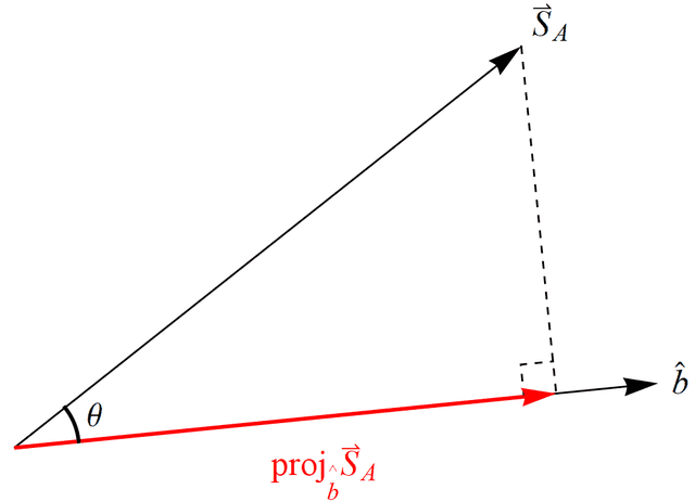
Figure 3. Projection of the angular momentum of Bob’s particle ##\vec{S}_B = \vec{S}_A## along the direction he chooses to measure it ##\hat{b}##. This does not happen with spin angular momentum.

Figure 4. Conservation of spin angular momentum for the spin triplet states in the plane of the conserved S = 1 vector. Reading from left to right, as Bob rotates his SG magnets relative to Alice’s SG magnets for her +1 outcome, the average value of his outcome varies from +1 (totally up, arrow tip) to 0 to –1 (totally down, arrow bottom). This obtains per conservation of spin angular momentum on average. Bob can say exactly the same about Alice’s outcomes as she rotates her SG magnets relative to his SG magnets for his +1 outcome. That is, their outcomes can only satisfy conservation of spin angular momentum on average, because they only measure +1/-1, never a fractional result as would be required for conservation to hold on a trial-by-trial basis for different measurements. The physical reason behind ##\theta = 2\Theta## is evident in this figure.
PhD in general relativity (1987), researching foundations of physics since 1994. Coauthor of “Beyond the Dynamical Universe” (Oxford UP, 2018).


Leave a Reply
Want to join the discussion?Feel free to contribute!