Blockworld and its Foundational Implications: General Relativity and the Big Bang

In parts 1 and 2 of this 5-part Insights series, I explained the blockworld (BW) implication of special relativity (SR). Geroch sums up the BW perspective nicely with this quote[1]:

There is no dynamics within space-time itself: nothing ever moves therein; nothing happens; nothing changes. In particular, one does not think of particles as moving through space-time, or as following along their world-lines. Rather, particles are just in space-time, once and for all, and the world-line represents, all at once, the complete life history of the particle.

Here in part 3 of this series, I will (conceptually) introduce general relativity (GR) and bring BW to bear on general relativistic cosmology to ‘explain’ what puzzles so many people about big bang cosmology (BBC), i.e., the origin of the universe. I should warn you that the answer will not be satisfying if you want an answer in terms of a time-evolved (dynamical) story because there is no time prior to the origin of the universe (big bang) to give rise dynamically to the big bang. This explanation in no way discounts the importance of research into resolving the singular nature of the big bang, I just want to bring the BW perspective to bear on the apparent special status of the origin of the universe. With that caveat, let me get this story started.

There are many ways to introduce GR, but I’m simply going to refer to its BW and local SR character, so my introduction will be conceptual. According to GR, spacetime isn’t flat, as in SR, but it’s curved and the timelike worldlines of objects in free fall (no non-gravitational forces) are geodesics in this curved spacetime. Let me unpack that statement a bit.

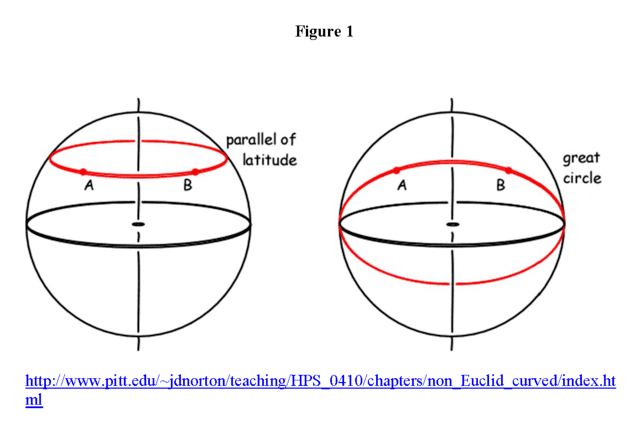
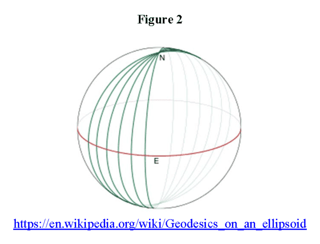
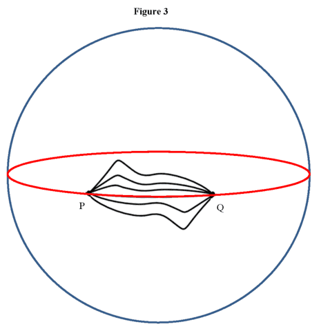
Geodesics are curves of extremal length. In a 2-dimensional (flat) plane, a geodesic is the curve of absolute shortest length between two points, i.e., the straight line connecting them. On the surface of a 2-dimensional sphere, geodesics are great circles, i.e., a circle on the sphere that shares its center with that of the sphere (Figures 1 & 2). All lines of longitude are geodesics, while the only line of latitude that is a geodesic is the equator (Figures 1 & 2). The short segment of the equator connecting points P and Q of Figure 3 is a path of absolute shortest length (the many paths shown nearby are all longer). The long segment of the equator connecting points P and Q of Figure 3 is a path of relative maximum length, i.e., paths nearby it are all a little shorter. The relative acceleration of neighboring geodetic worldlines depends on the curvature of the spacetime in their vicinity, so that spacetime curvature replaces gravity as a force. For example, two straight lines in a 2-dim plane emanating from a point continue to diverge at a constant rate because the space they’re in is flat. Conversely, the curvature of a 2-dim sphere means that two lines of longitude (geodesics) emanating south from the north pole diverge at an ever slower rate until at the equator they stop diverging and thereafter start to converge, eventually intersecting at the south pole. An object whose worldline is not a geodesic of the spacetime is under the influence of a (some) non-gravitational force(s).

So, the geometry of spacetime is an important thing to know and in GR it’s given by the “metric,” which gives the infinitesimal length squared anywhere in spacetime. For example, the metric on the 2-dim plane in Cartesian coordinates is

\begin{equation} ds^2 = dx^2 + dy^2   \label{metric1} \end{equation}

or in matrix form

\begin{equation} g_{\alpha \beta} = \begin{pmatrix} 1 & 0\\0 & 1 \end{pmatrix}   \label{metric2} \end{equation}

while the metric on the 2-dim sphere of radius r in spherical coordinates is

\begin{equation} ds^2 = r^2d\theta^2 + r^2 sin^2\theta d\phi^2   \label{metric3} \end{equation}

or in matrix form

\begin{equation} g_{\alpha \beta} = \begin{pmatrix} r^2 & 0\\0 & r^2sin^2\theta \end{pmatrix}   \label{metric4} \end{equation}

These can be used to compute the curvature of the plane or sphere, respectively, and thereby provide equations which can be solved for their geodesics. In order to obtain the metric, one must solve Einstein’s equations (EEs) of GR:

\begin{equation} G_{\alpha \beta} =  \frac{8 \pi G}{c^4} T_{\alpha \beta}  \label{EE1} \end{equation}

where [itex] G_{\alpha \beta} [/itex] is called the Einstein tensor and is a very complicated collection of [itex] g_{\alpha \beta} [/itex] to include its first and second derivatives in the four coordinates of spacetime. In fact, the LHS of EEs has thousands of [itex] g_{\alpha \beta} [/itex] terms when written in its most general form. Here is a quick overview to give you an idea of how complicated it is (you don’t need to follow in detailed fashion to get the idea).

\begin{equation} R_{\alpha \beta}\, – \frac{1}{2} g_{\alpha \beta} R =  \frac{8 \pi G}{c^4} T_{\alpha \beta}  \label{EE2} \end{equation}

where

\begin{equation} R = g^{\alpha \beta}R_{\alpha \beta} = g^{11}R_{11} + g^{12}R_{12}  + g^{13}R_{13} + … + g^{42}R_{42} +g^{43}R_{43} +g^{44}R_{44}     \label{R} \end{equation}

Whenever you see a repeated upper and lower index you have an implied summation over all four coordinate values (spacetime is 4-dimensional), so in general R (called the scalar curvature) contains 16 terms (10 independent terms since the inverse of the metric and the Ricci tensor are symmetric, i.e., [itex] g^{\alpha \beta} = g^{\beta \alpha}  [/itex] and [itex] R_{\alpha \beta} = R_{\beta \alpha}  [/itex]). Continuing we have the Ricci tensor [itex] R_{\alpha \beta} [/itex] constructed from the Riemann curvature tensor [itex] R^{\delta}_{\alpha \lambda \beta} [/itex] in these four terms

\begin{equation} R_{\alpha \beta} = R^{\lambda}_{\alpha \lambda \beta} \label{Ricci} \end{equation}

The Riemann curvature tensor is obtained from Christoffel symbols [itex] \Gamma^{\mu}_{\alpha \beta} [/itex]  as follows

\begin{equation} R^{\lambda}_{\alpha \tau \beta} = \frac{\partial \Gamma^{\lambda}_{\beta \alpha}}{\partial x^{\tau}} – \frac{\partial \Gamma^{\lambda}_{\tau \alpha}}{\partial x^{\beta}} + \Gamma^{\lambda}_{\tau \sigma} \Gamma^{\sigma}_{\beta \alpha} –  \Gamma^{\lambda}_{\beta \sigma} \Gamma^{\sigma}_{\tau \alpha} \label{Riemann} \end{equation}

which, because of the implied sums, contains 10 terms. And finally, each Christoffel symbol is constructed from the metric, its inverse and derivatives of the metric per

\begin{equation} \Gamma^{\mu}_{\alpha \beta} = \frac{g^{\mu \sigma}}{2} \left( \frac{\partial g_{\sigma \alpha}}{\partial x^{\beta}} + \frac{\partial g_{\sigma \beta}}{\partial x^{\alpha}} – \frac{\partial g_{\alpha \beta}}{\partial x^{\sigma}} \right)  \label{Christoffel} \end{equation}

an expression that contains 12 terms. That means Riemann has 1,176 terms in the metric, its inverse and derivatives of the metric, so Ricci has 4,704 such terms and R has 75,264 such terms. Not all the terms are independent, due to symmetries, but there are thousands of terms in the metric, its inverse, and its derivatives in the most general form of the Einstein tensor. In practice, the complexity is greatly reduced by finding solutions of EEs for highly symmetric spacetime metrics and stress-energy tensor [itex] T_{\alpha \beta} [/itex].

For example, Schwarzschild obtained the first solution of EEs the year after GR was published by finding the spacetime metric in the vacuum surrounding a spherically symmetric, static mass M. EEs in vacuum reduce to [itex] R_{\alpha \beta} = 0 [/itex] and if one starts with the most general spherically symmetric, static form of the metric

\begin{equation} ds^2 = -f(r)dt^2 + h(r)dr^2 + r^2d\theta^2 + r^2 sin^2\theta d\phi^2 \label{Schwarz} \end{equation}

and solves [itex] R_{\alpha \beta} = 0 [/itex] for f(r) and h(r), one obtains Schwarzschild’s solution

\begin{equation} ds^2 = -c^2 \left(1 – \frac{2GM}{c^2 r} \right)dt^2 + \left(1 – \frac{2GM}{c^2 r} \right)^{-1}dr^2 + r^2d\theta^2 + r^2 sin^2\theta d\phi^2 \label{Schwarz2} \end{equation}

In order to obtain the metric for BBC, we need to include the RHS of EEs with the stress-energy tensor (SET) that has the following general form:

\begin{equation} T_{\alpha \beta} = \begin{pmatrix} \mbox{energy density} & \mbox{momentum flux}\\ \mbox{momentum flux} & \mbox{stress or pressure} \end{pmatrix}   \label{SET1} \end{equation}

Notice that in order to provide the elements of the SET you have to know spatial and temporal distances for momentum, force, and energy. Of course, knowing that means you already know the metric. Therefore, you should view EEs equations as providing a self-consistency criterion or a “global constraint” between what you mean by spatial and temporal measurements and what you mean by momentum, force, and energy. Any combination of [itex] g_{\alpha \beta} [/itex]  and [itex] T_{\alpha \beta} [/itex]  that solves EEs constitutes a solution of GR.

There are some important facts about GR that I need to point out before proceeding. First, to do calculus on curved spaces (called “differentiable manifolds”), one assumes the manifold structure in small enough regions is essentially flat, so that calculus can be done piecewise on the manifold just as it’s done in flat space. The flat space results are connected between neighborhoods by, appropriately enough, “connections.” This means SR obtains locally in GR, bringing with it the BW ambiguity of a global “Now” (again, see The Fabric of the Cosmos: The Illusion of Time https://www.youtube.com/watch?v=vrqmMoI0wks for a nice conceptual explanation of BW). It also means there is no uniquely defined global conservation law. Instead we have SR’s local conservation of momentum and energy expressed as

\begin{equation} \nabla^{\alpha} G_{\alpha \beta} = \nabla^{\alpha} T_{\alpha \beta} = 0 \label{div} \end{equation}

Thus, the Einstein tensor and SET are said to be “divergence free.” This will have important implications for my discussion of closed timelike curves in part 4 of this Insights series.

Now we’re ready to describe the metric for BBC. Here, one makes assumptions that lead to a general metric form even simpler than that of Schwarzschild’s two unknown functions of one variable each, f(r) and h(r). One assumes that spacetime can be foliated into spatial hypersurfaces of homogeneity (same at every location) and isotropy (same in every direction) leading to a general metric form with just one unknown function of one variable a(t)

\begin{equation} ds^2 = -c^2dt^2 + a^2(t)( \mbox{spatial part}) \label{metricBBC} \end{equation}

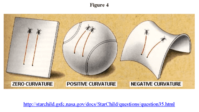
The spatial part can be a 3-dim flat space (zero curvature), 3-dim sphere (positive curvature), or 3-dim hyperboloid (negative curvature) (Figure 4).

The SET is that of a perfect fluid with either a pressureless dust with energy density [itex]\rho[/itex]  (called the “dust-filled” model)

\begin{equation} T_{\alpha \beta} = \begin{pmatrix} \rho & 0 & 0 & 0\\ 0 & 0 & 0 & 0\\0 & 0 & 0 & 0\\0 & 0 & 0 & 0  \end{pmatrix}   \label{SET2} \end{equation}

or radiation with isotropic pressure p (called the “radiation-filled” model)

\begin{equation} T_{\alpha \beta} = \begin{pmatrix} \rho & 0 & 0 & 0\\ 0 & p & 0 & 0\\0 & 0 & p & 0\\0 & 0 & 0 & p  \end{pmatrix}   \label{SET3} \end{equation}

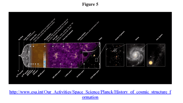
EEs are then solved for [itex] a(t) [/itex]. In the flat case, [itex] \dot a(t \rightarrow \infty) \rightarrow 0 [/itex], i.e., the universe is expanding at ‘escape velocity’ and will expand forever at an ever slower rate that approaches zero as t approaches infinity. The hyperboloid will also expand forever, but with an asymptotic growth rate larger than zero, i.e.,  [itex] \dot a(t \rightarrow \infty) \gt 0 [/itex]. The spherical universe will grow to a maximum size then shrink to zero. In all three scenarios, tracing the evolution of [itex] a(t) [/itex] backwards in time [itex] a(0) [/itex] is chosen to be zero, the so-called “big bang,” i.e., the origin of the universe (Figure 5). For example, in the Einstein-de Sitter (EdS) cosmology model (aka the flat, matter-dominated model) EEs give the following differential equation for [itex] a(t) [/itex]

\begin{equation} 2\ddot a a + \dot a^2 = 0 \label{EdS} \end{equation}

Since this is a second-order differential equation, its general solution will contain two arbitrary constants. Typically those constants are specified by choosing [itex] a(0) = 0 [/itex] and [itex] a(t_o) = 1 [/itex] where [itex] t_o [/itex] is the age of the universe, i.e., [itex] a(t_o) = 1 [/itex] is the current value of the scaling factor. In that case, we have [itex] a(t) = (\frac{t}{t_o})^{2/3} [/itex]. However, one could chose a non-zero value for [itex] a(0) [/itex] so that [itex] a(t) = (\frac{t + B}{t_o + B})^{2/3} [/itex]. In that case, [itex] a(0) = (\frac{B}{t_o + B})^{2/3} [/itex] where [itex] B [/itex] is chosen to specify [itex] a(0) \neq 0 [/itex]. The problem with choosing [itex] a(0) [/itex] is that we don’t have an external agent to justify our choice. Typically, when solving a physics problem we know the initial conditions because some external agent implements them. But, when the system in question is the entire universe, there is no external agent to implement the initial conditions. Thus, the initial conditions are inexplicable, dynamically speaking. This is not a problem for adynamical explanation, as we will now see.

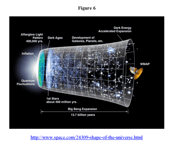
Notice that the solution of EEs for BBC can also be viewed as a BW (Figure 5). As Geroch says, “nothing ever moves therein; nothing happens; nothing changes” in this BW view. While the solution depicted in Figure 5 was created in time-evolved fashion (Smolin[2] calls this mathematics the “Newtonian Schema”) the solution itself, i.e., self-consistent metric and SET on the spacetime manifold, is just a ‘static’ entity. In this BW view, the existence of any point in Figure 5 is no more surprising than any other. The big bang is unique in that it’s a singular point, meaning the solution of GR breaks down there. But, we assume quantum gravity will replace that singularity with a well-behaved event, e.g., a quantum fluctuation as in Figure 6, or, again, we could choose [itex] a(0) \neq 0 [/itex]. Regardless, the origin of the universe (big bang) is just one point in the BW and as such its existence is no more mysterious than any other point of the BW. The reason the big bang seems mysterious is that a dynamical story about the universe traced backwards in time ends at the big bang. The state of the universe at any given time t is explained dynamically by time evolving the state of the universe at the time immediately preceding t. Finding and using the laws that govern time evolution form the basis of dynamical explanation. Since there is no time preceding the big bang and there are no external agents to implement initial conditions for the universe as a whole, the big bang (or [itex] a(0) \neq 0 [/itex]) cannot be explained dynamically.

We are dynamic creatures, our perceptions are formed in time-evolved fashion, so we’re predisposed to think dynamically and, therefore, we want to understand/explain what we experience dynamically. However, it may be that physics is telling us that despite our time-evolved perceptions, dynamical explanation is not fundamental. This possibility will be more evident in part 5 of this series when I talk about quantum nonlocality. As we will see, in all such cases, mysteries such as the origin of the universe arise because our time-evolved bias demands dynamical explanation. The key to avoiding this explanatory problem is to relegate dynamical explanation based on time-evolved stories to secondary (non-fundamental) status and accept that the more general BW explanation based on a spatiotemporally global constraint is truly fundamental. Wharton[3] calls this the “Lagrangian Schema Universe.” In this more general BW view of explanation, EEs are understood adynamically as a global constraint, a self-consistency criterion for the metric and SET on the spacetime manifold. While time-evolved stories can certainly be told in GR solutions, there well may be events in a GR solution that resist such dynamical explanation, e.g., the big bang. In those cases, we just have to accept that reality is best understood adynamically in spatiotemporally holistic fashion. As Wharton says[3],

When examined critically, the Newtonian Schema Universe assumption is exactly the sort of anthropocentric argument that physicists usually shy away from. It’s basically the assumption that the way we humans solve physics problems must be the way the universe actually operates.

In the next (fourth) part of this 5-part series, I will bring this BW view of GR to bear on the paradoxes associated with closed timelike curves.

1. Geroch, R.: General Relativity from A to B. University of Chicago Press, Chicago (1978), pp 20-21.

2. Smolin, L.: The unique universe: Against the timeless multiverse. Physics World, 21–26 (June 2009).

3. Wharton, K.: The Universe is not a Computer. In Questioning the Foundations of Physics, A. Aguirre, B. Foster and Z. Merali (Eds), pp.177-190, Springer (2015)  http://arxiv.org/abs/1211.7081. This essay won third prize in the 2012 FQXi essay contest.