Blockworld and its Foundational Implications: General Relativity and Closed Timelike Curves

In parts 1 and 2 of this 5-part Insights series, I explained the blockworld (BW) implication of special relativity (SR). In part 3, I introduced general relativity (GR) and brought BW to bear on general relativistic cosmology to ‘explain’ what puzzles so many people about big bang cosmology, i.e., the origin of the universe. The bottom line there was that we just have to accept that reality is best understood adynamically in spatiotemporally holistic fashion, giving up[1] “the assumption that the [Newtonian Schema] way we humans solve physics problems must be the way the universe actually operates.” Here in part 4 of this series, I will bring this idea to bear on the paradoxes associated with GR’s closed timelike curves (CTCs).

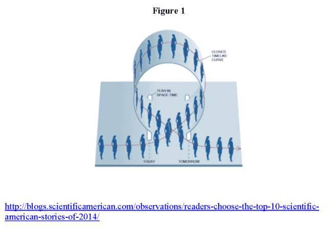
Recall from part 3 that objects in free fall have timelike geodetic worldlines in the GR spacetime. Using a vacuum solution of Einstein’s equations (EEs) we can find its geodesics and imagine it harboring a small object where “small” means that it doesn’t change the spacetime geometry appreciably. For example, this is done for GPS satellites in the Schwarzschild solution in order to correct for different clocks rates between Earth-bound clocks and orbiting clocks[2 & 3]. Indeed, as Ashby says[2], “If these relativistic effects were not corrected for, satellite clock errors building up in just one day would cause navigational errors of more than 11 km, quickly rendering the system useless.” As it turns out, there are some GR spacetimes that possess timelike geodesics that loop back onto themselves, i.e., CTCs (Figure 1). For example, Gott found a well-known example using cosmic strings[4]. This can happen because GR employs curved spacetime manifolds and EEs are solved locally on that manifold. Thus, one can construct a spacetime satisfying EEs whereby time is forward directed locally along a path while that path bends around globally into the past. This leads to two types of paradoxes[5], i.e., consistency paradoxes and causal loops.

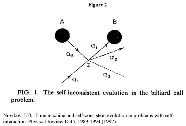
Consistency paradoxes are those like the “grandfather paradox,” i.e., someone goes into the past and kills his grandfather before he was born, thereby preventing his own birth. A simpler version of that paradox that I will discuss herein is from Novikov (Figure 2), whereby a wormhole connects regions A and B such that a ball going into region B at time T on trajectory α₁ comes out of region A at an earlier time T – ΔT on trajectory α₂ so that it strikes itself at point Z, scattering in two directions, α₂ and α₃. But, neither α₂ nor α₃ enters region B, so in fact, the ball never enters region B to come out of region A to strike itself at point Z, which is a contradiction.

Causal loops provide for the existence of something that doesn’t have an origin. For example, in the movie “Back to the Future,” Marty McFly enjoys playing guitar in 1984. One of his favorite songs to play is Chuck Berry’s hit “Johnny B. Goode” released in 1958. Marty time travels back to 1955 and plays the song at a dance where Chuck Berry’s cousin, Marvin Berry, hears the song and calls Chuck to let him hear it. So, Chuck Berry got the song from Marty McFly in 1955, released it in 1958, Marty McFly hears it in 1984, time travels to 1955, and plays it for Chuck Berry to hear. So, who actually wrote “Johnny B. Goode?”

These are the paradoxes I will address via the BW, adynamical global constraint view of reality. This in no way discounts the important research concerning technical issues associated with the existence of CTCs[6]. I just want to bring the BW perspective to bear on the paradoxes of CTCs.

As with the other puzzle and conundrums I’m writing about in this series, the paradoxes associated with CTCs arise because our time-evolved bias demands dynamical explanation. That is, as dynamic creatures our perceptions are formed in time-evolved fashion, so we’re predisposed to think dynamically and, therefore, we want to understand reality as we experience it. In the context of CTCs, we can imagine paradox-generating initial conditions, e.g., rolling the ball on trajectory α₁ in Figure 2, so we’re genuinely mystified as to how Nature will respond to that situation when our best dynamical laws say a violation of logic will result. The short answer might be, “All laws of physics obey the laws of logic. Assuming a phenomenon must satisfy the laws of physics in order to occur, all logic violating phenomena are ruled out as being possible.” Along these lines we have Novikov’s Principle of Self-Consistency[7] which states simply that local solutions of the laws of physics are only permissible if they lead to self-consistent global solutions. Carlini et al. showed[8] in fact that Novikov’s Principle of Self-Consistency actually follows from the principle of least action, which is precisely the “Lagrangian Schema” mathematical approach to physics advocated by Wharton in part 3 (cited above). So, let me expand on the Lagrangian versus the Newtonian Schema.

The Newtonian Schema (NS) is the mathematical approach corresponding to what I’ve been calling “dynamical explanation.” One inputs initial conditions (the initial state of the system in question) and a dynamical law tells you how that initial state is time-evolved to some final state. Sean Carroll sums it up nicely in this quote[9]:

Let’s talk about the actual way physics works, as we understand it. Ever since Newton, the paradigm for fundamental physics has been the same, and includes three pieces. First, there is the “space of states”: basically, a list of all the possible configurations the universe could conceivably be in. Second, there is some particular state representing the universe at some time, typically taken to be the present. Third, there is some rule for saying how the universe evolves with time. You give me the universe now, the laws of physics say what it will become in the future. This way of thinking is just as true for quantum mechanics or general relativity or quantum field theory as it was for Newtonian mechanics or Maxwell’s electrodynamics.

As Carroll points out, all the theories of physics can be written in the NS. In contrast, the Lagrangian Schema (LS) says the behavior of objects isn’t due to forces governing their behavior instant by instant, but rather their behavior from start to finish is the result of a minimal (extremal) action. The action S is the Lagrangian L integrated over the time interval in question,

\begin{equation} S = \int L \, dt \label{action} \end{equation}

where L is the difference between the system’s kinetic and potential energies, so S is a spatiotemporally global quantity. The dynamical laws of the NS follow for each infinitesimal time dt in the LS when you demand [itex] \delta S = 0 [/itex], i.e., that S is extremal. EEs are actually the NS version of the following action

\begin{equation} S = \int \left[ \frac{c^4}{16 \pi G} R + \mathcal{L}_M \right] \, \sqrt{-g} \, d^4x \label{action2} \end{equation}

where R is the scalar curvature, [itex] \mathcal{L}_M [/itex] is the matter-energy Lagrangian density, and [itex] \sqrt{-g} \, d^4x [/itex] is the invariant spacetime volume element. That EEs are an NS formulation of GR leads some to view GR dynamically instead of in BW fashion which then fuels the CTC paradoxes. A la Carlini et al., if you rather take the LS approach, EEs are best understood as an adynamical global constraint and one must find a metric and stress-energy tensor (SET) on the entire spacetime manifold in order to have a GR solution.

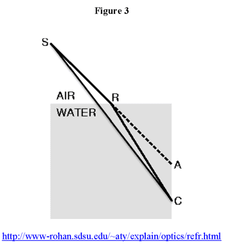
An easy way to see the difference between the NS (dynamical view) and the LS (BW view) is to consider the example of a light ray emitted from point S in air and arriving at point C in water (Figure 3). The explanation per the LS is that the path S to R to C is the path of least time. The direct path S to C (shown) takes longer, so it’s not the path taken. The NS explanation is that the light ray emitted from S towards R proceeds without deviation, since nothing is interacting with it, until it hits the water at point R. The water then refracts the light towards point C. While both methods yield the same result, we tend to favor the NS explanation, since the LS explanation sounds a bit like the light ray intended to go to C and calculated its path based on the presence of the water. According to the NS, the light ray that reached C was refracted at R, otherwise it would’ve gone to point A, i.e., it didn’t adjust its emission direction with the intention of reaching C and it certainly doesn’t ‘know’ it will encounter water when it’s emitted. But the BW view doesn’t attribute any intentionality or prescience to the light ray, rather it simply relegates dynamical explanation to secondary status a priori. If you want to know why something happens the way it does, the fundamental reason has to do with a spatiotemporally holistic characterization of the phenomenon under investigation. If the subsequent BW analysis permits it, a time-evolved story can be told in conjunction with the BW explanation. Otherwise, the fundamental BW explanation just does not permit a dynamical story, so the BW explanation just has to be accepted as the final answer.

Returning to CTCs, if you have a solution of EEs that permits a causal loop and there is no reason to believe you couldn’t instantiate that solution, e.g., it doesn’t require a SET that we have no way of producing, then you would just have to accept the fact that not everything has an origin. The belief that everything like a song must have an origin is clearly a bias based on our dynamical experience.

But, you say, what about the consistency paradox of Figure 2? Exactly how am I stopped from rolling the ball on trajectory α₁? Is there a ‘physics police’ who will arrest me before I can do so? Will I be struck by lightning? These are questions based on the spatiotemporally local NS problem solving method that aligns so well with our dynamical experience. The answer is, you have to adopt the BW view and use the LS problem solving method which says a GR solution isn’t a solution unless it accounts for the entire spacetime manifold M. Piecewise local solutions to EEs are worthless in and of themselves. When you imagined sitting in the spacetime of Figure 2 and rolling the ball on trajectory α₁, you were making an assumption that clearly doesn’t hold true. You were assuming, for all practical purposes, that the spacetime geometry of Figure 2 would not change due to your presence, just as the vacuum Schwarzschild spacetime geometry doesn’t change due to the presence of a GPS satellite. So, as with the satellite in the Schwarzschild solution, you just ignored the SET associated with the ball. In the Schwarzschild solution that’s ok, because you can certainly create a SET for the satellite in orbit that is everywhere divergence free and well-defined on M. Remember, the SET is a requirement of EEs

\begin{equation} G_{\alpha \beta} =  \frac{8 \pi G}{c^4} T_{\alpha \beta}  \label{EE1} \end{equation}

even though it doesn’t seem to affect the metric on the LHS. If you want to introduce an object to M, you have to construct the corresponding SET element for the RHS of EEs, no matter how seemingly innocuous that object is geometrically speaking. Otherwise, you don’t have a GR solution. And, if you imagine a situation that is ruled out by GR such as the paradoxical trajectory α₁ of Figure 2, then it’s ruled out by physics. So, finally, we have resolved the consistency paradox resulting from the spatiotemporally local, dynamical view by adopting the spatiotemporally global BW view of GR. We end up turning the original question on its NS inquisitor by telling him that if he wants to know what will happen in Figure 2, he will have to construct a GR solution that embodies his premises as well as consequences. For example, Echeverria et al. did precisely that with similar cases[10] by simply varying the time delay created by the wormhole on the otherwise contradictory trajectory, thus creating a self-consistent solution for a trajectory starting along α₁ in Figure 2. In that case, the answer to the question posed by our NS inquisitor is that the result of rolling the ball on the trajectory α₁ will be a self-consistent solution as shown by Echeverria.

In the next (fifth) part of this 5-part series, we will see that the conundrums of quantum nonlocality support the BW view even more strongly than the CTC paradoxes.

1. Wharton, K.: The Universe is not a Computer. In Questioning the Foundations of Physics, A. Aguirre, B. Foster and Z. Merali (Eds), pp.177-190, Springer (2015)  http://arxiv.org/abs/1211.7081. This essay won third prize in the 2012 FQXi essay contest.

2. Ashby, N.: Relativity and the Global Positioning System. Physics Today 55, 41-47 (2002).

3. For details of geodesic computations see the derivations of equations 29 and 42 in Stuckey, W.M.: The Schwarzschild black hole as a gravitational mirror. American Journal of Physics 61, 448-456 (1993).

4. Gott, J.R.: Closed timelike curves produced by pairs of moving cosmic strings: Exact solutions. Physical Review Letters 66, 1126-1129 (1991).

5. Lobo, F.: Closed timelike curves and causality violation. Classical and Quantum Gravity: Theory, Analysis and Applications, Chapter 6, Nova Science Publishers (2008) http://arxiv.org/abs/1008.1127

6. For example, Morris, M., Thorne, K., and Yurtsever, U.: Wormholes, Time Machines, and the Weak Energy Condition. Physical Review Letters 61, 1446-1449 (1988); Mikheeva, E., and Novikov, I.D.: Inelastic billiard balls in a spacetime with a time machine. Physical Review D 47, 1432-1436 (1993); Goldwirth, D., Perry, M., Piran, T., and Thorne, K.: Quantum propagator for a nonrelativistic particle in the vicinity of a time machine. Physical Review D 49, 3951-3957 (1994).

7. Novikov, I.D.: An analysis of the operation of a time machine. Soviet Physics JETP 68, 439-443 (1989).

8. Carlini, A., Frolov, V.P., Mensky, M.B., Novikov, I.D., and Soleng, H.H.: Time machines: the Principle of Self-Consistency as a Consequence of the Principle of Minimal Action. International Journal of Modern Physics D4, 557-580 (1995) http://arxiv.org/abs/gr-qc/9506087

9. Carroll, S.: A Universe from Nothing? Discover Magazine Online (28 Apr 2012) http://blogs.discovermagazine.com/cosmicvariance/2012/04/28/a-universe-from-nothing/

10. Echeverria, F., Klinkhammer, G., & Thorne, K.: Billiard balls in wormhole spacetimes with closed timelike curves: Classical theory. Physical Review D 44, 1077-1099 (1991).

Note: Comments for this post have been disabled. Please show your feedback by using the star rating at the top of the article and or contacting the author personally.