Dark Energy Part 1: Einstein-deSitter Cosmology

In this 3-part series, I want to motivate the (re)introduction of the cosmological constant ##\Lambda## into Einstein’s equations of general relativity (GR) per the Supernova Cosmology Project (SCP) Union2.1 type Ia supernova data. As you probably know, this discovery won Perlmutter, Schmitt, and Riess the 2011 Nobel Prize in Physics “for the discovery of the accelerating expansion of the Universe through observations of distant supernovae.” ##\Lambda## is referred to as “dark energy” and as we will see in Part 2 it leads to the accelerating expansion of the universe. In this Insight (Part 1 of the series), I will introduce Einstein-deSitter (EdS) cosmology. In Part 2, I will introduce ##\Lambda##CDM cosmology (essentially EdS + ##\Lambda##). In Part 3, I will introduce the notion of distance modulus in astronomy and fit the SCP Union2.1 type Ia supernova data (distance modulus versus redshift) with both of these models. This will make it clear why astronomers began to take seriously the need for ##\Lambda## even though Einstein had earlier retracted his introduction of ##\Lambda## as “the greatest blunder of my career.” Let’s begin!

To review from my Insight General Relativity and the Big Bang, Einstein’s equations (EEs) of GR are:

\begin{equation} G_{\alpha \beta} =  \frac{8 \pi G}{c^4} T_{\alpha \beta}  \label{EE1} \end{equation}

where ##G_{\alpha \beta}## is called the Einstein tensor and is a very complicated collection of the spacetime metric ## g_{\alpha \beta} ## to include its first and second derivatives in the four coordinates of spacetime (see below). In fact, the LHS of EEs has thousands of ## g_{\alpha \beta} ## terms when written in its most general form. But, cosmology solutions of EEs make simplifying assumptions which greatly reduce the complexity. In fact, we will have only two ordinary differential equations in two functions of one variable for EdS and ##\Lambda##CDM cosmologies. Expanding ##G_{\alpha \beta}## in Eq. (\ref{EE1}) into its constituent terms we have

\begin{equation} R_{\alpha \beta}\, – \frac{1}{2} g_{\alpha \beta} R =  \frac{8 \pi G}{c^4} T_{\alpha \beta}  \label{EE2} \end{equation}

where R is the scalar curvature and is given by the Ricci tensor ##R_{\alpha \beta}## as follows

\begin{equation} R = g^{\alpha \beta}R_{\alpha \beta} = g^{11}R_{11} + g^{12}R_{12}  + g^{13}R_{13} + … + g^{42}R_{42} +g^{43}R_{43} +g^{44}R_{44}     \label{R} \end{equation}

Whenever you see a repeated upper and lower index you have an implied summation over all four coordinate values (spacetime is 4-dimensional, 4D). ##g^{\alpha \beta}## is the inverse of the metric ##g_{\alpha \beta}##, which is what we want to solve EEs to find. In EdS cosmology, one assumes that 4D spacetime can be foliated into flat spatial hypersurfaces of homogeneity (same at every location) and isotropy (same in every direction). With these simplifying assumptions, the metric can be written with just one unknown function of one variable ##a(t)## in Cartesian coordinates as

\begin{equation} ds^2 = -c^2dt^2 + a^2(t)(dx^2 + dy^2 + dz^2) \label{metricEdS} \end{equation}

To picture what this metric describes, imagine a balloon with a coordinate grid drawn on it. As the balloon inflates or deflates, the size of the grid increases or decreases, respectively, but the “co-moving” coordinate distance between any two points remains the same.

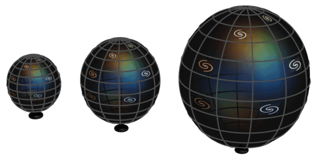
To get the actual distance from the coordinate distance, you would need to multiply the coordinate distance by a “scaling factor,” that scaling factor is ##a(t)##. The non-zero components of the metric are then ##g_{00} = -c^2## and ##g_{11} = g_{22} = g_{33} = a^2(t)## where the coordinates ##x^{\alpha}## are ##x^0 = t##, ##x^1 = x##, ##x^2 = y##, and ##x^3 = z##. Thus, the non-zero components of ##g^{\alpha \beta}## are ##g^{00} = \frac{-1}{c^2}## and ##g^{11} = g^{22} = g^{33} = \frac{1}{a^2(t)}##.

Now, to finish setting up EEs we need to compute the Ricci tensor ##R_{\alpha \beta}## by contracting indices of the Riemann curvature tensor ##R^{\lambda}_{\alpha \tau \beta}##

\begin{equation} R_{\alpha \beta} = R^{\lambda}_{\alpha \lambda \beta} = \frac{\partial \Gamma^{\lambda}_{\beta \alpha}}{\partial x^{\lambda }} – \frac{\partial \Gamma^{\lambda}_{\lambda \alpha}}{\partial x^{\beta}} + \Gamma^{\lambda}_{\lambda \sigma} \Gamma^{\sigma}_{\beta \alpha} –  \Gamma^{\lambda}_{\beta \sigma} \Gamma^{\sigma}_{\lambda \alpha} \label{Ricci}  \end{equation}

where the Christoffel symbol ##\Gamma^{\mu}_{\alpha \beta}## is constructed from the inverse of the metric and derivatives of the metric per

\begin{equation} \Gamma^{\mu}_{\alpha \beta} = \frac{g^{\mu \sigma}}{2} \left( \frac{\partial g_{\sigma \alpha}}{\partial x^{\beta}} + \frac{\partial g_{\sigma \beta}}{\partial x^{\alpha}} – \frac{\partial g_{\alpha \beta}}{\partial x^{\sigma}} \right)  \label{Christoffel} \end{equation}

These equations account for the LHS of EEs ##G_{\alpha \beta}##, so now we need the stress-energy tensor ##T_{\alpha \beta}## (SET) for the RHS. Given the assumed symmetry of the metric, the SET must be that of a perfect fluid. Einstein and deSitter assumed the pressure of that perfect fluid is zero, leaving only one non-zero term in ##T_{\alpha \beta}## for a pressureless dust with energy density ##\rho## (called a “dust-filled” model)

\begin{equation} T_{\alpha \beta} = \begin{pmatrix} \rho & 0 & 0 & 0\\ 0 & 0 & 0 & 0\\0 & 0 & 0 & 0\\0 & 0 & 0 & 0  \end{pmatrix}   \label{SET} \end{equation}

There are then only two independent EEs in the two functions ##a(t)## and ##\rho(t)##

\begin{equation} R_{00}\, – \frac{1}{2} g_{00} R =  8 \pi T_{00} = 8\pi \rho  \label{EEtime} \end{equation}

and

\begin{equation} R_{11}\, – \frac{1}{2} g_{11} R =  8 \pi T_{11} = 0  \label{EEspace} \end{equation}

where I am using “geometrized units” ##G = c = 1##. Using these equations, we find

\begin{equation} R_{00} = -3 \frac{\ddot{a}}{a}   \label{R00} \end{equation}

\begin{equation} R_{11} = \ddot{a}a + 2\dot{a}^2  \label{R11} \end{equation}

\begin{equation} R = 6 \frac{\ddot{a}}{a} + 6 \frac{\dot{a}^2}{a^2}  \label{ScalarR} \end{equation}

giving these two differential equations to be solved for ##a(t)## and ##\rho(t)##

\begin{equation} 3 \frac{\dot{a}^2}{a^2} = 8\pi\rho   \label{E1} \end{equation}

\begin{equation} -2\ddot{a} a – \dot{a}^2 = 0 \label{E2} \end{equation}

Eq. (\ref{E2}) can be written

\begin{equation} \frac{d}{dt}\left(\dot{a}^2a\right) = 0 \label{E2a} \end{equation}

so that ##\left(\dot{a}^2a\right)## is a constant. Multiplying Eq. (\ref{E1}) by ##a^3## gives us

\begin{equation} 3\left(\dot{a}^2a\right) = 8\pi \rho a^3 \label{E1a} \end{equation}

Thus, we see that ##\rho a^3## is a constant, which makes sense because it simply means that the amount of mass in a co-moving volume of space remains fixed (see Section 3.1 in this Insight by Arman777). We’re not concerned with the exact functional form for ##\rho(t)##, we’re only concerned with finding ##a(t)## and we get that from solving Eq. (\ref{E2}). That’s an ordinary second-order differential, so the particular solution requires two boundary conditions. The standard choice is ##a(0) = 0## and ##a(t_o) = 1## where ##t_o## is the current value of the coordinate time ##t## which is the proper time for co-moving observers (those with fixed coordinate position). ##t_o## is therefore taken to be the age of the universe. Eq. (\ref{E2}) is separable via Eq. (\ref{E2a}), so this is very easy to solve giving ##a(t) = \left(\frac{t}{t_0}\right)^{2/3}##. This tells us that the universal acceleration is always negative and growing to zero as ##t \rightarrow \infty##, since

\begin{equation} \ddot{a} = -\frac{2}{9}\left(\frac{1}{t_o}\right)^{2/3}\frac{1}{t^{4/3}} \label{EdSaccel} \end{equation}

It’s analogous to an object being ejected at escape velocity (see Part 3 in this Insight by Arman777). We’ll compare this to the situation in ##\Lambda##CDM cosmology in Part 2 of this series where we will see that ##\ddot{a}## in that case starts negative but changes to positive. That happened when the universe was about 54% of its current age for our universe (see p. 6 in this publication). Now let us use our solution for ##a(t)## to find some kinematics between co-moving observers who exchange photons.

Without loss of generality, we may assume we are at the coordinate origin receiving the photon from some distant co-moving emitter on the ##x## axis. The “proper distance” between us at ##x = 0## and a co-moving emitter at ##x = X_e## is ##r(t) = a(t)X_e##, as I explained earlier. That is to say, if you stopped the expansion of the universe at time ##t## and traveled from ##x = 0## to ##x = X_e##, then you would have travelled a distance of ##a(t)X_e## (see Section 2.1 in this Insight by Arman777). We will compute the proper distance ##r_o := r(t_o)## to ##X_e## when the photon is received, the proper distance ##r_e := r(t_e)## to ##X_e## when the photon was emitted, the time ##t_e## when the photon was emitted, the Hubble recession velocity of the emitter today ##v_o := \frac{dr}{dt}\left(t_o\right)##, and the Hubble recession velocity of the emitter when the photon was emitted ##v_e := \frac{dr}{dt}\left(t_e\right)## as functions of the redshift ##z## of the photon and age of the universe ##t_o##.

The redshift of the photon is given by (see Section 2.2 in this Insight by Arman777)

\begin{equation} z = \frac{\lambda_r – \lambda_e}{\lambda_e} = \frac{a_o – a_e}{a_e} \rightarrow z + 1 = \frac{a_o}{a_e} = \frac{1}{a_e} \label{redshift}\end{equation}

where of course

\begin{equation} a_e = \left(\frac{t_e}{t_o}\right)^{2/3} \label{ae} \end{equation}

Eqs. (\ref{redshift}) and (\ref{ae}) immediately give us

\begin{equation} t_e = \frac{t_0}{\left(1+z\right)^{1.5}} \label{te} \end{equation}

By definition, we have ##r_o = a_oX_e = X_e##. To get ##X_e## we note that the photon takes a null path from ##X_e## to ##x = 0##, i.e., ##ds^2 = 0## for the photon path. The metric then gives us

\begin{equation} ds^2 = 0 = -c^2dt^2 + a^2(t)dx^2 \label{photon} \end{equation}

for the photon path. This means

\begin{equation} \int_{t_e}^{t_o}\frac{cdt}{a} = -\int_{X_e}^{0} dx = X_e  \label{Xeqn} \end{equation}

noting that the photon is moving in the negative ##dx## direction. Eq. (\ref{Xeqn}) with Eq. (\ref{ae}) then give us

\begin{equation} X_e = 3ct_o\left(1 – \left(\frac{t_e}{t_o}\right)^{1/3}\right) = 3ct_o\left(1 – \frac{1}{\sqrt{1+z}}\right) \label{X}\end{equation}

Accordingly, the farthest points we can see (we could have received a photon from) would be at ##r_o = 3ct_o## today, corresponding to an infinitely redshifted photon emitted at ##t = 0## and received only today at ##t = t_o##. That distance ##3ct_o## is called the “particle horizon” aka “the edge of the observable universe” (see this Insight by Arman777). Notice that the particle horizon is three times farther away than the distance the photon traversed, i.e., ##ct_o## corresponding to a local photon speed ##c## times ##t_o##. That’s because space is expanding while the photon is moving towards us, so much of the space between us and the emitter was created behind the photon as it made its journey.

To get the distance to the emitter at time ##t_e## we have

\begin{equation} r_e = a_eX_e = a_er_o = \frac{r_o}{1+z} \label{re} \end{equation}

To get the Hubble recession velocity of a co-moving observer at ##x = X## relative to us, we have

\begin{equation} v(t) = \frac{dr}{dt} = \dot{a}(t)X = \frac{\dot{a}}{a}aX = H(t)r(t) \label{hubblelaw}\end{equation}

Eq. (\ref{hubblelaw}) is called “Hubble’s law” and ##H = \frac{\dot{a}}{a}## is the Hubble parameter (see Part 2 in this Insight by Arman777). The value of the Hubble parameter today is called the Hubble constant and denoted ##H_o##. Plugging ##t = t_o## into Eq. (\ref{hubblelaw}) we obtain

\begin{equation} v_o = \left(\frac{1}{t_o}\right)^{2/3}\frac{2}{3}t_o^{-1/3}X_e = \frac{2r_o}{3t_o} = 2c\left(1 – \frac{1}{\sqrt{1+z}}\right) \label{vo}  \end{equation}

Thus, objects at the edge of the observable universe are receding at twice the speed of light. This does not violate special relativity, which continues to hold locally in GR. Here is a nice article explaining this and other misconceptions about Big Bang cosmology that appeared in Scientific American in 2005. Finally, to get ##v_e## we have

\begin{equation} v(t_e) = \dot{a}(t_e)X_e = \left(\frac{1}{t_o}\right)^{2/3}\frac{2}{3}t_e^{-1/3}X_e = \frac{2r_o}{3t_o}\left(\frac{t_o}{t_e}\right)^{1/3} = v_o\sqrt{1+z} \label{ve} \end{equation}

As an example, let us evaluate the kinematics for a galaxy with redshift of ##z## = 11.9 discovered in 2012 (see article here). We’ll use ##t_o## = 13.82Gy, obtained from the Planck telescope in 2013 (see article here). Note that “Gy” is read “billion years,” since G = ##10^9## and y stands for “years.”  Plugging ##t_o## and ##z## into Eq. (\ref{X}) we obtain ##r_o## = 29.9Gcy, which is about 72% of the way to the particle horizon, 41.5Gcy away. Here, “Gcy” is read “billion light-years,” since G = ##10^9##, ##c## is the speed of light, and y stands for “years.” These conventions make the kinematical equations easy to use. Eq. (\ref{re}) gives us ##r_e## = 2.32Gcy, Eq. (\ref{vo}) gives us ##v_o = 1.44c##, Eq. (\ref{ve}) gives us ##v_e = 5.18c##, and Eq. (\ref{te}) gives us ##t_e## = 0.298Gy = 298My (where M = ##10^6## so “My” is read “million years”).

So, the complete picture is as follows. The image we are seeing in the 2012 article was emitted when the universe was only 298 million years-old by a primitive galaxy that was 2.32 billion light-years away from the infant Milky Way. That primitive galaxy was being carried away from our location at a speed of over 5 times the speed of light by the expansion of the universe. Today, as we receive the image, the universe is 13.82 billion years-old and that galaxy is presumably a mature galaxy located 29.9 billion light-years from us and it is being carried away from our location at a speed of 1.44 times the speed of light by the expansion of the universe.

In Part 2 of this series, I will solve EEs for the counterparts to these EdS kinematics when a cosmological constant ##\Lambda## is added to the EdS assumptions. In Part 3, I will explain the concept of distance modulus and use these cosmology models to fit the SCP Union2.1 type Ia supernova data. This will show why astronomers began to believe that a cosmological constant is necessary.

Continue to Part 2

Comment Thread