Dark Energy Part 2: LCDM Cosmology

This is Part 2 of a 3-part series explaining evidence for so-called “dark energy” leading to a current positive cosmological acceleration. The evidence comes from fitting the SCP Union2.1 type Ia supernova data which indicates the existence of a cosmological constant ##\Lambda## (read “Lambda”, thus ##\Lambda##CDM is sometimes written LCDM) in Einstein’s equations (EEs) of general relativity (GR). This ##\Lambda## is referred to as “dark energy” and creates a current positive cosmological acceleration, as we will see below. This is in stark contrast to what we found in Part 1 for Einstein-deSitter (EdS) cosmology (a spatially flat, dust-filled cosmology model). There I showed that the cosmological acceleration in EdS cosmology is always negative. I will use some of the results from Part 1 here to obtain EdS plus ##\Lambda##, aka ##\Lambda##CDM, where “CDM” stands for “cold dark matter.” ##\Lambda##CDM is the currently accepted and most widely used cosmology model, i.e., the concordance model of cosmology. In Part 3, I will fit the SCP Union2.1 data with both models showing how the EdS fit is greatly improved with the addition of ##\Lambda##. Let’s get started!

Our new EEs are

\begin{equation} R_{\alpha \beta}\, – \frac{1}{2} g_{\alpha \beta} R + \Lambda g_{\alpha \beta} =  \frac{8 \pi G}{c^4} T_{\alpha \beta}  \label{EE} \end{equation}

Again, using geometrized units G = c = 1, the EdS EEs are changed to

\begin{equation} 3 \frac{\dot{a}^2}{a^2} + g_{00}\Lambda = 8\pi\rho   \label{E1} \end{equation}

\begin{equation} -2\ddot{a} a – \dot{a}^2 + a^2\Lambda = 0 \label{E2} \end{equation}

Eq. (\ref{E2}) gives

\begin{equation} \frac{d}{dt}\left(\dot{a}^2a\right) = a^2\dot{a}\Lambda \label{E2a} \end{equation}

Multiplying Eq. (\ref{E1}) by ##a^3## we obtain

\begin{equation} \left(\dot{a}^2a\right) – \Lambda\frac{a^3}{3} = \frac{8}{3}\pi \rho a^3 \label{E1a} \end{equation}

Taking ##\frac{d}{dt}## of Eq. (\ref{E1a}) we obtain

\begin{equation} \frac{d}{dt}\left(\dot{a}^2a\right) – a^2\dot{a}\Lambda = \frac{8}{3}\pi \frac{d}{dt}\left(\rho a^3\right) \label{E2b} \end{equation}

Thus, Eq. (\ref{E2a}) in Eq. (\ref{E2b}) tells us that ##\rho a^3## is a constant, just like in EdS cosmology. That makes sense, since we expect the mass in a co-moving volume to remain fixed regardless of ##\Lambda##.

Putting current values into Eq. (\ref{E1}) we obtain

\begin{equation} 3 H_o^2 – \Lambda = 8\pi\rho_o \rightarrow \frac{8\pi\rho_o}{3 H_o^2} + \frac{\Lambda}{3 H_o^2} = 1   \label{E1now} \end{equation}

where I used ##a_o = 1## and ##H(t) = \frac{\dot{a}}{a}##, as explained in Part 1. Defining ##\Omega_m := \frac{8\pi\rho_o}{3 H_o^2}## and ##\Omega_\Lambda := \frac{\Lambda}{3 H_o^2}## we have

\begin{equation} \Omega_m + \Omega_\Lambda = 1 \label{OmOL}\end{equation}

Rewriting Eq. (\ref{E1}) as

\begin{equation} \dot{a} = \sqrt{\frac{8\pi\rho a^3}{3a} + \frac{a^2\Lambda}{3}} \label{adot1}\end{equation}

and using ##\rho a^3 = \rho_o## with our definitions of ##\Omega_m## and ##\Omega_\Lambda##, Eq. (\ref{adot1}) becomes

\begin{equation} \dot{a} = H_o\sqrt{\frac{\Omega_m}{a} + \Omega_\Lambda a^2} \label{adot}\end{equation}

Eqs. (\ref{E1now}) and (\ref{OmOL}) suggest ##\Lambda## be viewed as a source of gravity just like ##\rho##. However, since we can’t “see” this source it is “dark” and referred to as “dark energy.” Below, I will show that it leads to accelerating expansion in contrast to ##\rho## which we saw in Part 1 leads to decelerating expansion only. We can use these equations to find the kinematics between photon exchangers in ##\Lambda##CDM cosmology. Eq. (\ref{adot}) gives us

\begin{equation} \int \frac{da}{\sqrt{\frac{\Omega_m}{a} + \Omega_\Lambda a^2}} = H_o\int dt \label{Hot}\end{equation}

Using Eq. (\ref{Hot}) we obtain the following two equations

\begin{equation} \int_0^1 \frac{da}{\sqrt{\frac{\Omega_m}{a} + \Omega_\Lambda a^2}} = H_ot_o \label{Hoto}\end{equation}

\begin{equation} \int_{a_e}^1 \frac{da}{\sqrt{\frac{\Omega_m}{a} + \Omega_\Lambda a^2}} = H_o\left(t_o – t_e \right) \label{Hote}\end{equation}

which we can solve numerically given ##\Omega_m## (or equivalently ##\Omega_\Lambda##) and ##z## (recall, ##a_e = \frac{1}{1+z}##). I will supply a MATLAB program at the conclusion of this Insight for all computations. Note: @GeorgeJones found an analytic solution to Eq. (\ref{Hot}):

\begin{equation} \int \frac{da}{\sqrt{\frac{\Omega_m}{a} + \Omega_\Lambda a^2}} = \frac{2}{3\sqrt{\Omega_\Lambda}}\mbox{sinh}^{-1}\left(\sqrt{\frac{\Omega_\Lambda}{\Omega_m}}a^{3/2}\right) + \mbox{Constant} \end{equation}

I’ll do the integral numerically, since it’s actually easier to type the integral into MATLAB than it is to type this solution. But, it is pretty mathematics, so I wanted to include it. We can use Eqs. (\ref{Hoto}) and (\ref{Hote}) to obtain

\begin{equation} \frac{t_e}{t_o} = \frac{H_ot_o – H_o\left(t_o – t_e\right)}{H_ot_o} \label{te}\end{equation}

This will give us ##t_e##. Now, as with EdS shown in Part 1, we have

\begin{equation} \int_{t_e}^{t_o}\frac{cdt}{a} = -\int_{X_e}^{0} dx = X_e  \label{Xeqn} \end{equation}

for the emission of a photon at time ##t_e## from co-moving position ##x = X_e## that is received today at time ##t_o## and co-moving position ##x = 0##. Unlike EdS, EEs for ##\Lambda##CDM don’t give us ##a(t)##, so I will rewrite Eq. (\ref{Xeqn}) as an integral in ##a## using Eq. (\ref{adot}) and ##dt = \frac{da}{\dot{a}}##

\begin{equation} X_e = \frac{ct_o}{H_ot_o}\int_{a_e}^{1}\frac{da}{a\sqrt{\frac{\Omega_m}{a} + \Omega_\Lambda a^2}}  \label{ro} \end{equation}

So, Eq. (\ref{ro}) gives us an equation we can solve numerically for the proper distance ##r_o = X_e## (as explained in Part 1) to the photon emitter today. Again, all we need are either ##\Omega## and the redshift ##z##. We obtain the current Hubble recession velocity of the photon source via ##v_o = H_or_o##

\begin{equation} v_o = c\int_{a_e}^{1}\frac{da}{a\sqrt{\frac{\Omega_m}{a} + \Omega_\Lambda a^2}}  \label{vo} \end{equation}

Just as with EdS cosmology, we have

\begin{equation} r_e = a_eX_e = \frac{r_o}{1 + z} \label{re} \end{equation}

So, we have only to obtain ##v_e##. For that we have

\begin{equation} v_e = X_e \dot{a}(t_e) = X_eH_o\sqrt{\frac{\Omega_m}{a_e} + \Omega_\Lambda a_{e}^2} = v_o\sqrt{\Omega_m (1+z) + \frac{\Omega_\Lambda}{(1+z)^2}} \label{ve} \end{equation}

which reduces to the relationship between ##v_e## and ##v_o## in the EdS model with ##\Omega_m = 1## as we would expect.

Finally, I will compute the ##\Lambda##CDM kinematics for the galaxy with redshift of ##z## = 11.9 that I analyzed in Part 1 with EdS kinematics. Again, I will use ##t_o## = 13.82Gy. Here is my MATLAB code:

%These are the two functions in the scaling factor “a” that I will be integrating. Om is ##\Omega_m## and OL is ##\Omega_\Lambda##.
%I have it ready to accept a string of “a” values as will be necessary for the Union2.1 data in Part 3.
Afunc = @(a,Om,OL) 1./sqrt(Om./a + OL*a.^2);
Rfunc = @(a,Om,OL) 1./sqrt(Om.*a + OL*a.^4);

%These are currently accepted values for ##\Omega_m## and ##\Omega_\Lambda##. They will be fitting parameters for the Union2.1 data in Part 3.
Om = 0.29;
OL = 1 – Om;

%This is the age of the universe in Gy.
to = 13.82;

%Our redshift.
z = 11.9;

%This is the numerical integral for ##H_o## times ##t_o##.
Hoto = integral(@(a) Afunc(a,Om,OL),0,1)

%This is ##a_e##. Again, I have it ready to accept a string of z values as will be necessary for the Union2.1 data in Part 3.
ae = 1./(1 + z);

%This is the numerical integral for ##H_o(t_o – t_e)##.
Hotote = integral(@(a) Afunc(a,Om,OL),ae,1);

%This is ##t_e## in Gy.
te = to*(1 – Hotote/Hoto)

%This is the numerical integral for ##r_o## in Gcy.
Ro = to*integral(@(a) Rfunc(a,Om,OL),ae,1)/Hoto

%This is ##v_o## in c.
Vo = Hoto*Ro/to

%This is ##r_e## in Gcy.
Re = Ro/(1+z)

%This is ##v_e## in c.
Ve = Vo/Afunc(ae,Om,OL)

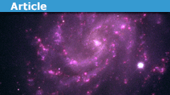
I obtained the following results (EdS results in ( ) next to the ##\Lambda##CDM results). The image we are seeing in the 2012 article was emitted when the universe was only 379 (298) million years-old by a primitive galaxy that was 2.55 (2.32) billion light-years away from the infant Milky Way. That primitive galaxy was being carried away from our location at a speed of 4.48 (5.18) times the speed of light by the expansion of the universe. Today, as we receive the image, the universe is 13.82 billion years-old and that galaxy is presumably a mature galaxy located 32.9 (29.9) billion light-years from us and it is being carried away from our location at a speed of 2.32 (1.44) times the speed of light by the expansion of the universe.

To conclude, as I warned in Part 1, I point out that ##\Lambda## causes the acceleration of the universe to change from negative to positive. Taking ##\frac{d}{dt}## of Eq. (\ref{adot}) we obtain

\begin{equation} \ddot{a} = \frac{H_{0}^2}{2}\left(-\frac{\Omega_m}{a^2} + \Omega_\Lambda 2a \right) \label{addot} \end{equation}

Eq. (\ref{addot}) reduces to what I found for EdS cosmology in Part 1 for ##\ddot{a}## when ##\Omega_m = 1## (which means ##\Omega_\Lambda = 0##) and ##a = \left(\frac{t}{t_o}\right)^{2/3}##. What we see in this equation is that when ##a## was small, the ##-\frac{\Omega_m}{a^2}## term dominates making ##\ddot{a}## negative. Thus, early in the history of the universe ##\rho## dominated the acceleration rate making the universe decelerate (negative acceleration). However, as ##a## grows larger the term ##\Omega_\Lambda 2a ## eventually equals the term ##-\frac{\Omega_m}{a^2}## and ##\ddot{a} = 0##. After that ##\Lambda## dominates the acceleration rate making the universe accelerate instead of decelerate. Solving for when that happens we find

\begin{equation} a = \left(\frac{\Omega_m}{2\Omega_\Lambda}\right)^{1/3}  \label{addotzero} \end{equation}

Using ##a = \frac{1}{1+z}##, ##\Omega_m## = 0.3, ##\Omega_\Lambda## = 0.7, and Eqs. (\ref{Hoto}), (\ref{Hote}), and (\ref{te}) gives us ##z## = 0.671 and ##\frac{t_e}{t_o}## = 0.544, i.e., the universe stopped decelerating and started accelerating when it was 54% of its current age (as I stated in Part 1). [See p. 6 of this publication.]

In Part 3, I will explain the concept of distance modulus and use the EdS and ##\Lambda##CDM cosmology models to fit the SCP Union2.1 type Ia supernova data. This will show why astronomers began to believe that a cosmological constant is necessary and won Perlmutter, Schmitt, and Riess the 2011 Nobel Prize in Physics.

Continue to Part 3

Comment Thread