Examples of Prequantum Field Theories II: Higher Gauge Fields

After having recalled ordinary gauge fields from a dg-algebraic perspective in the previous article, here I discuss how in these terms we easily get the concept of higher (nonabelian) gauge fields, i.e. of gauge fields whose “vector potential” is not just a 1-form but involves differential forms of higher degree. These will be the fields of the prequantum Chern-Simons type fields theories to be discussed in the next article.

Ordinary gauge fields are characterized by the property that there are no non-trivial gauge-of-gauge transformations, equivalently that their BRST complexes contain no higher-order ghosts. Mathematically, it is natural to generalize beyond this case to higher gauge fields, which do have non-trivial higher gauge transformations.

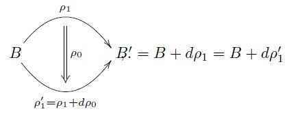
The simplest example is a “2-form field” (B-field), generalizing the “vector potential” 1-form ##A## of the electromagnetic field. Where such a 1-form has gauge transformations given by 0-forms (functions) ##\kappa## via $$A \stackrel{\kappa}{\longrightarrow} A’ = A +d\kappa\,,$$ a 2-form ##B## has gauge transformations given by 1-forms ##\rho_1##, which themselves then have gauge-of-gauge-transformations given by 0-forms ##\rho_0##:

Next a “3-form field” (C-field’) has third order gauge transformations:

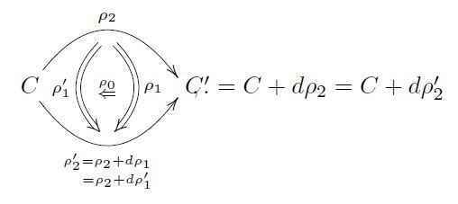
Similarly “##n##-form fields” have order-##n## gauge-of-gauge transformations and hence have order-##n## ghost-of-ghosts in their BRST complexes.

Higher gauge fields have not been experimentally observed, to date, as fundamental fields of nature, but they appear by necessity and ubiquitously in higher-dimensional supergravity and in the hypothetical physics of strings and ##p##-branes. The higher differential geometry which we develop is to a large extent motivated by making precise and tractable the global structure of higher gauge fields in string and M-theory.

Generally, higher gauge fields are part of mathematical physics just as the Ising model and ##\phi^4##-theory are, and as such, they do serve to illuminate the structure of experimentally verified physics.

For instance, the Einstein equations of motion for ordinary (bosonic) general relativity on 11-dimensional spacetimes are equivalent to the full super-torsion constraint in 11-dimensional supergravity with its 3-form higher gauge field [CandielloLechner 93].  From this point of view, one may regard the 3-form higher gauge field in supergravity, together with the gravitino, as auxiliary fields that serve to present Einstein’s equations for the graviton in a particularly neat mathematical way.

We now use the above dg-algebraic formulation of ordinary gauge fields from the previous article in order to give a quick but accurate idea of the mathematical structure of higher gauge fields.

Above we saw that (finite-dimensional) Lie algebras are equivalently the formal duals of those differential graded-commutative algebras whose underlying graded commutative algebra is freely generated from a (finite-dimensional) vector space over the ground field. From this perspective, there are two evident generalizations to be considered: we may take the underlying vector space to already have contributions in higher degrees itself, and we may pass from vector spaces, being modules over the ground field ##\mathbb{R}##, to (finite rank) projective modules over an algebra of smooth functions on a smooth manifold.

Hence we say that an ##L_\infty##-algebroid (of finite type) is a smooth manifold ##X## equipped with a ##\mathbb{N}##-graded vector bundle (degreewise of finite rank), whose smooth sections hence form an ##\mathbb{N}##-graded projective ##C^\infty(X)##-module ##\mathfrak{a}_\bullet##, and equipped with an ##\mathbb{R}##-linear differential ##d_{\mathrm{CE}}## on the Grassmann algebra of the ##C^\infty(X)##-dual ##\mathfrak{a}^\ast## modules
$$
\mathrm{CE}(\mathfrak{a})
:=
\left(
\wedge^\bullet_{C^\infty(X)}(\mathfrak{a}^\ast),
\;
d_{\mathrm{CE}(\mathfrak{a})}
\right)
\,.
$$
Accordingly, a homomorphism of ##L_\infty##-algebroids we take to be a dg-algebra homomorphism (over ##\mathbb{R}##) of their CE-algebras going the other way around. Hence the category of ##L_\infty##-algebroids is the full subcategory of the opposite of that of differential graded-commutative algebras over ##\mathbb{R}## on those whose underlying graded-commutative algebra is free on graded locally free projective ##C^\infty(X)##-modules:
$$
L_\infty\mathrm{Algbd}
\hookrightarrow
\mathrm{dgcAlg}^\mathrm{op}
\,.
$$
We say we have a Lie n-algebroid when ##\mathfrak{a}_\bullet## is concentrated in the lowest ##n##-degrees. Here are some important examples of ##L_\infty##-algebroids:

When the base space is the point, ##X = \ast##, and ##\mathfrak{a} ## is concentrated in degree 0, then
we recover Lie algebras. Generally, when the base space is the point, then the ##\mathbb{N}##-graded module ##\mathfrak{a}##
is just an ##\mathbb{N}##-graded vector space ##\mathfrak{g}##. We write ##\mathfrak{a} = \mathbf{B}\mathfrak{g}## to indicate this, and then ##\mathfrak{g}## is an L-infinity algebra. When in addition ##\mathfrak{g}## is concentrated in the lowest ##n## degrees, then these are also called Lie n-algebras. With no constraint on the grading but assuming that the differential sends single generators always to sums of wedge products of at most two generators, then we get dg-Lie algebras.

The Weil algebra of a Lie algebra ##\mathfrak{g}## hence exhibits a Lie 2-algebra. We may think of this as the Lie 2-algebra
##\mathrm{inn}(\mathfrak{g})## of inner derivations of ##\mathfrak{g}##. By the above discussion, it is suggestive to write ##\mathbf{E}\mathfrak{g}## for this Lie 2-algebra, hence
$$
\mathrm{W}(\mathbf{B}\mathfrak{g}) = \mathrm{CE}(\mathbf{B}\mathbf{E}\mathfrak{g})
\,.
$$

If ##\mathfrak{g} = \mathbb{R}[n]## is concentrated in degree ##p## on the real line (so that the CE-differential is necessarily trivial), then we speak of the line Lie (p+1)-algebra ##\mathbf{B}^p \mathbb{R}##, which as an ##L_\infty##-algebroid over the point is to be denoted
$$
\mathbf{B}\mathbf{B}^{p}\mathbb{R} = \mathbf{B}^{p+1}\mathbb{R}
\,.
$$

All this goes through verbatim, up to additional signs, with all vector spaces generalized to super-vector spaces. The Chevalley-Eilenberg algebras of the resulting super L-infinity algebras are known in parts of the supergravity literature
“FDA“s. This had been the topic of the previous articles Homotopy Lie n-algebras in supergravity and Emergence from the superpoint.

Passing now to ##L_\infty##-algebroids over non-trivial base spaces, first of all, every smooth manifold ##X## may be regarded as the ##L_\infty##-algebroid over ##X##, these are the Lie 0-algebroids. We just write ##\mathfrak{a} = X## when the context is clear.

For the tangent bundle ##T X## over ##X## then the graded algebra of its dual sections is the wedge product algebra of differential forms,
##\mathrm{CE}(T X ) = \Omega^\bullet(X)## and hence the de Rham differential makes ##\wedge^\bullet \Gamma(T^\ast X)## into a dgc-algebra and hence makes ##T X## into a Lie algebroid. This is called the tangent Lie algebroid of ##X##. We usually write ##\mathfrak{a} = TX## for the tangent Lie algebroid (trusting that context makes it clear that we do not mean the Lie 0-algebroid over the underlying manifold of the tangent bundle itself). In particular this means that for any other ##L_\infty##-algebroid ##\mathfrak{a}## then flat ##\mathfrak{a}##-valued differential forms on some smooth manifold ##\Sigma## are equivalently homomorphisms of ##L_\infty##-algebroids like so:
$$
\Omega_{\mathrm{flat}}(\Sigma,\mathfrak{a})
\;\;=\;\;
\left\{
\; T \Sigma \longrightarrow \mathfrak{a}\;
\right\}
\,.
$$
In particular ordinary closed differential forms of degree ##n## are equivalently flat ##\mathbf{B}^n\mathbb{R}##-valued differential forms:
$$
\Omega^n_{\mathrm{cl}}(\Sigma)
\;\; \simeq \;\;
\left\{
\; T \Sigma \longrightarrow \mathbf{B}^n \mathbb{R}\;
\right\}
\,.
$$

More generally, for ##\mathfrak{a}## any ##L_\infty##-algebroid over some base manifold ##X##, then we have its Weil dgc-algebra
$$
\mathrm{W}(\mathfrak{a})
:=
\left(
\wedge^\bullet_{C^\infty(X)}( \mathfrak{a}^\ast \oplus \Gamma(T^\ast X) \oplus \mathfrak{a}^\ast[1] ),
d_{\mathrm{W}} = d_{\mathrm{CE}} + \mathbf{d} )
\right)
\,,
$$
where ##\mathbf{d}## acts as the degree shift isomorphism in the components ##\wedge^1_{C^\infty(X)}\mathfrak{a}^\ast \longrightarrow \wedge^1_{C^\infty(X)}\mathfrak{a}^\ast[1]## and as the de Rham differential in the components ##\wedge^k \Gamma(T^\ast X) \to \wedge^{k+1}\Gamma(T^\ast X)##. This defines a new ##L_\infty##-algebroid that may be called the tangent ##L_\infty##-algebroid ##T \mathfrak{a}##
$$
\mathrm{CE}(T \mathfrak{a}) := \mathrm{W}(\mathfrak{a})
\,.
$$
We also write ##\mathbf{E}\mathbf{B}^p \mathbb{R}## for the ##L_\infty##-algebroid with
$$
\mathrm{CE}(\mathbf{E}\mathbf{B}^p \mathbb{R})
:=
\mathrm{W}(\mathbf{B}^{p}\mathbb{R})
\,.
$$

In direct analogy with the discussion for Lie algebras, we then say that an unconstrained ##\mathfrak{a}##-valued differential form ##A## on a manifold ##\Sigma## is a dg-algebra homomorphism from the Weil algebra of ##\mathfrak{a}## to the de Rham dg-algebra on ##\Sigma##:
$$
\Omega(\Sigma,\mathfrak{a})
:=
\left\{
\; \Omega^\bullet(\Sigma) \longleftarrow \mathrm{W}(\mathfrak{a}) \;
\right\}
\,.
$$

For ##G## a Lie group acting on ##X## by diffeomorphisms, then there is the action Lie algebroid ##X/\mathfrak{g}## over ##X## with ##\mathfrak{a}_0 = \Gamma_X(X \times \mathfrak{g})## the ##\mathfrak{g}##-valued smooth functions over ##X##. Write ##\rho : \mathfrak{g} \to \mathrm{Vect}## for the linearized action. With a choice of basis ##\{t_a\}## for ##\mathfrak{g}## as before
and assuming that ##X = \mathbb{R}^n## with canonical coordinates ##x^i##, then ##\rho## has components ##\{\rho_a^\mu\}## and the CE-differential on ##\wedge^\bullet_{C^\infty(X)} (\Gamma_X(X \times \mathfrak{g}^\ast))## is given on generators by
$$
\begin{aligned}
d_{\mathrm{CE}} &: f \mapsto t^a \rho_a^\mu \partial_\mu f
\\
d_{\mathrm{CE}} &: t^a \mapsto \tfrac{1}{2}C^{a}{}_{b c} t^b \wedge t^c
\end{aligned}
\,.
$$
In the physics literature this Chevalley-Eilenberg algebra ##\mathrm{CE}(X/\mathfrak{g})## is known as the BRST complex of ##X## for infinitesimal symmetries ##\mathfrak{g}##. If ##X## is thought of as a space of fields, then the ##t_a## are called ghost fields.

Given any ##L_\infty##-algebroid, it induces a whole bouquet of further ##L_\infty##-algebroids via extension by higher cocycles.
A ##p+1##-cocycle on an ##L_\infty##-algebroid ##\mathfrak{a}## is a closed element
$$
\mu \in (\wedge^\bullet_{C^\infty(X)}\mathfrak{a}^\ast)_{p+1} \hookrightarrow \mathrm{CE}(\mathfrak{a})
\,.
$$
Notice that now cocycles are representable by the higher line ##L_\infty##-algebras ##\mathbf{B}^{p+1}\mathbb{R}## from above:
$$
\begin{aligned}
\left\{
\mu \in \mathrm{CE}(\mathfrak{a})_{p+1} \;|\; d_{\mathrm{CE}}\mu = 0
\right\}
&
\simeq
\left\{
\;
\mathrm{CE}(\mathfrak{a})
\stackrel{\mu^\ast}{\longleftarrow}
\mathrm{CE}(\mathbf{B}^{p+1}\mathbb{R})
\;
\right\}
\\
& =
\left\{
\;
\mathfrak{a} \stackrel{\mu}{\longrightarrow} \mathbf{B}^{p+1}\mathbb{R}
\;
\right\}
\end{aligned}
\,.
$$

It is a traditional fact that ##\mathbb{R}##-valued 2-cocycles on a Lie algebra induce central Lie algebra extensions. More generally,
higher cocycles ##\mu## on an ##L_\infty##-algebroid induce ##L_\infty##-extensions ##\hat {\mathfrak{a}}##, given by the pullback

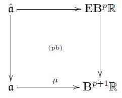
Equivalently this makes ##\hat{\mathfrak{a}}## be the homotopy fiber of ##\mu## in the homotopy theory of ##L_\infty##-algebras, and induces a long homotopy fiber sequence of the form

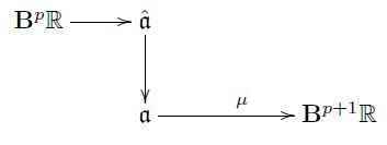
In components this means simply that ##\mathrm{CE}(\hat{\mathfrak{a}})## is obtained from ##\mathrm{CE}(\mathfrak{a})## by adding one generator ##c## in degre ##p## and extending the differential to it by the formula
$$
d_{\mathrm{CE}} : c = \mu
\,.
$$
This construction has a long tradition in the supergravity literature, we discussed this before in Emergence form the superpoint.

For example for ##\mathfrak{g}## a semisimple Lie algebra with binary invariant polynomial ##\langle -,-\rangle## (the Killing form), then ##\mu_3 = \langle-,[-,-]\rangle## is a 3-cocycle. The ##L_\infty##-extension by this cocycle is a Lie 2-algebra called the string Lie 2-algebra ##\mathfrak{string}_\mathfrak{g}##. If ##\{t^a\}## is a linear basis of ##\mathfrak{g}^\ast## as before write ##k_{a b} := \langle t_a, t_b\rangle## for the components of the Killing form; the components of the 3-cocycle are ##\mu_{a b c} = k_{a a’}C^{a’}{}_{b c}##. The CE-algebra of the string Lie 2-algebra then is that of ##\mathfrak{g}## with a generator ##b## added and with CE differential defined by
$$
\begin{aligned}
d_{\mathrm{CE}(\mathfrak{string})} & : t^a \mapsto \tfrac{1}{2}C^a{}_{b c} t^b \wedge t^c
\\
d_{\mathrm{CE}(\mathfrak{string})} & : b \mapsto k_{a a’}C^{a’}{}_{c b} t^a \wedge t^b \wedge t^c
\,.
\end{aligned}
$$
Hence a flat ##\mathfrak{string}_{\mathfrak{g}}##-valued differential form on some ##\Sigma## is a pair consisting of an ordinary flat ##\mathfrak{g}##-valued 1-form ##A## and of a 2-form ##B## whose differential has to equal the evaluation of ##A## in the 3-cocoycle:
$$
\Omega_{\mathrm{flat}}(\Sigma,\mathfrak{string}_{\mathfrak{g}})
\;\simeq\;
\left\{
(A,B) \in \Omega^1(\Sigma,\mathfrak{g})\times\Omega^2(\Sigma)
\;|\;
F_A = 0 \,,\;\; d B = \langle A \wedge [A \wedge A]\rangle
\right\}
\,.
$$
Notice that since ##A## is flat, the 3-form ##\langle A \wedge [A \wedge A]\rangle## is its Chern-Simons 3-form. More generally, Chern-Simons forms are such that their differential is the evaluation of the curvature of ##A## in an invariant polynomial.

An invariant polynomial ##\langle -\rangle## on an ##L_\infty##-algebroid we may take to be a ##d_{\mathrm{W}}##-closed element in the shifted generators of its Weil algebra ##\mathrm{W}(\mathfrak{a})##
$$
\langle -\rangle \in \wedge^\bullet_{C^\infty(X)}(\mathfrak{a}^\ast[1]) \hookrightarrow \mathrm{W}(\mathfrak{a})
\,.
$$
When one requires the invariant polynomial to be binary, i.e. in ##\wedge^2 (\mathfrak{a}^\ast[1]) \to \mathrm{W}(\mathfrak{a})## and non-degenerate, then it is also called a shifted symplectic form and it makes ##\mathfrak{a}## into a symplectic Lie n-algebroid. For ##n = 0## these are the symplectic manifolds, for ##n = 1## these are called Poisson Lie algebroids, for ##n = 2## they are called Courant Lie 2-algebroids \cite{RoytenbergCourant}. There are also plenty of non-binary invariant polynomials.

Being ##d_{\mathrm{W}}##-closed, an invariant polynomial on ##\mathfrak{a}## is represented by a dg-homomorphism:
$$
W(\mathfrak{a}) \longleftarrow \mathrm{CE}(\mathbf{B}^{p+2}\mathbb{R}) : \langle – \rangle
$$
This means that given an invariant polynomial ##\langle -\rangle## for an ##L_\infty##-algebroid ##\mathfrak{a}##, then it assigns to any ##\mathfrak{a}##-valued differential form ##A## a plain closed ##(p+2)##-form ##\langle F_A\rangle## made up of the ##\mathfrak{a}##-curvature forms, namely the composite
$$
\Omega^\bullet(\Sigma)
\stackrel{A}{\longleftarrow}
W(\mathfrak{a})
\stackrel{\langle -\rangle}{\longleftarrow} \mathrm{CE}(\mathbf{B}^{p+2}\mathbb{R}) : \langle F_A \rangle
\,.
$$
In other words, ##A## may be regarded as a nonabelian pre-quantization of $\langle F_A\rangle$.

Therefore we may consider now the ##\infty##-groupoid of ##\mathfrak{a}##-connections whose gauge transformations preserve the specified invariant polynomial, such as to guarantee that it remains a globally well-defined differential form. The smooth ##\infty##-groupoid of ##\mathfrak{a}##-valued connections with such gauge transformations between them we write ##\exp(\mathfrak{a})_{\mathrm{conn}}##. As a smooth simplicial presheaf, it is hence given by the following assignment:

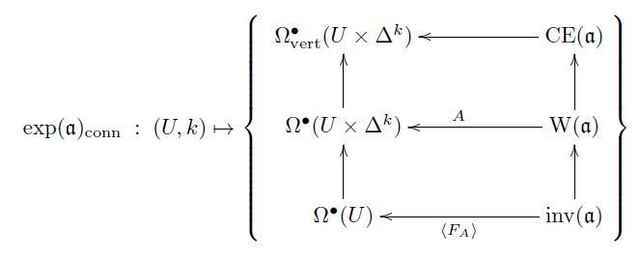
Here on the right we have, for every ##U## and ##k##,  the set of those ##A## on ##U \times \Delta^k## that induce gauge transformations along the ##\Delta^k##-direction (that is the commutativity of the top square) such that the given invariant polynomials evaluated on the curvatures are preserved (that is the commutativity of the bottom square).

This ##\exp(\mathfrak{a})_{\mathrm{conn}}## is the moduli stack of ##\mathfrak{a}##-valued connections with gauge transformations
and gauge-of-gauge transformations between them that preserve the chosen invariant polynomials.

The key example is the moduli stack of ##(p+1)##-form gauge fields
$$
\exp(\mathbf{B}^{p+1}\mathbb{R})_{\mathrm{conn}}/\mathbb{Z}
\simeq
\mathbf{B}(\mathbb{R}/_{\!\hbar}\mathbb{Z})_{\mathrm{conn}}
$$

Generically we write
$$
\mathbf{A}_{\mathrm{conn}} := \mathrm{cosk}_{n+1} (\exp(\mathfrak{a})_{\mathrm{conn}})
$$
for the ##n##-truncation of a higher smooth stack of ##\mathfrak{a}##-valued gauge field connections obtained this way. If ##\mathfrak{a} = \mathbf{B}\mathfrak{g}## then we write ##\mathbf{B}G_{\mathrm{conn}}## for this.

Given such, then an ##\mathfrak{a}##-gauge field on ##\Sigma## (an ##\mathbf{A}##-principal connection) is equivalently a map of smooth higher stacks
$$
\nabla : \Sigma \longrightarrow \mathbf{A}_{\mathrm{conn}}
\,.
$$
By the above discussion, a simple map like this subsumes all of the following component data:

• a choice of open cover ##\{U_i \to \Sigma\}##;
• a ##\mathfrak{a}##-valued differential form ##A_i## on each chart ##U_i##;
• on each intersection ##U_{i j}## of charts a path of infinitesimal gauge symmetries whose integrated finite gauge symmetry ##g_{i j}## takes ##A_i## to ##A_j##;
• on each triple intersection ##U_{i j k}## of charts a path-of-paths of infinitesimal gauge symmetries whose integrated finite gauge-of-gauge symmetry takes the gauge transformation ##g_{i j}\cdot g_{j k}## to the gauge transformation ##g_{i k}##
• and so on.

Hence a ##\mathfrak{a}##-gauge field is locally ##\mathfrak{a}##-valued differential form data which are coherently glued together to a global structure by gauge transformations and higher-order gauge-of-gauge transformations.

Given two globally defined ##\mathfrak{a}##-valued gauge fields this way, then a globally defined gauge transformation them is equivalently a homotopy between maps of smooth higher stacks

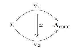
Again, this concisely encodes a system of local data: this is on each chart ##U_i## a path of infinitesimal gauge symmetries whose integrated gauge transformation transforms the local ##\mathfrak{a}##-valued forms into each other, together with various higher-order gauge transformations and compatibilities on higher-order intersections of charts.

Then a gauge-of-gauge transformation is a homotopy of homotopies

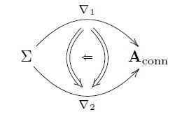
and again this encodes a recipe for how to extract the corresponding local differential form data.

For more on all these constructions, see [Sati-Schreiber-Stasheff 09] [Fiorenza-Schreiber-Stasheff 10] [Fiorenza-Rogers-Schreiber 11].

In conclusion, the correct higher field bundle for ##\mathfrak{a}##-gauge theory is the stacky bundle of the form

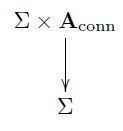
(see also the exposition at Higher field bundles for gauge fields). The next article discusses how from transgressive cocycles on ##L_\infty##-algebroids one may construct prequantum field theory Lagrangians on such field bundles.

Click For Forum Comments