Learn the Fundamentals of the Diffraction Grating Spectrometer

Introduction

In this article we will discuss the fundamentals of the diffraction grating spectrometer.  The operation of the instrument is based upon the textbook equations for the far-field interference (Fraunhofer case) that results from a plane wave incident on a diffraction grating.   It is rather remarkable how the standard textbook equations can be used to tell most everything one needs to know in order to understand the complete operation of the instrument.  It is hoped that upon reading this article, the reader will have a good understanding of how a diffraction grating spectrometer works.

For a diffraction grating spectrometer, the grating is the dispersive element instead of a prism.  In very simple form, the primary maxima from a diffraction grating for wavelength ## \lambda ## are found at angles ## \theta ## that satisfy ## m \lambda=d \sin{\theta}  ##, with ##m=## integer.  The result is different wavelengths (or colors) will emerge from the grating at different angles. For a beginner, this is the basics of how the diffraction grating spectrometer works.  One of our goals here is to be able to compute the resolution capabilities ## \Delta \lambda ## of the instrument.  We will look at the operation in full detail, with an equation that will not only give us info on the location of the primary maxima, but also info on the angular spread (linewidth) of the primary maxima.  From that we can determine whether it is the width of the entrance slit that is determining the instrument’s resolution ## \Delta \lambda ##, or if the entrance slit is sufficiently narrow that the angular spread of the primary maximum due to diffraction is responsible for the observed linewidth from a perfectly monochromatic source.

Components and Optical Layout

The diffraction grating is normally a reflective type grating,  rather than of the transmissive type.  The principles are the same,  where the lines or grooves on the grating  can be thought of as Huygens mirrors.  The grating will typically have a line density ## \delta ## of about 1000 vertical lines or grooves on it per millimeter, and typical dimensions are about 2″ square ,(50 mm), so that the total number of lines ## N ## on the grating can be as many as 50,000 or more.  The number ## N ## will be used in calculations below to estimate the diffraction limit of the resolution  (spectral linewidth) ## \Delta \lambda ## that can be achieved. Note that the distance ## d ## between lines or grooves on the grating is ## d=\frac{1}{\delta} ##.

In order to have a plane wave incident on the grating,  the instrument has an entrance slit that lies in the focal plane of a concave spherical mirror, which makes for a collimated beam (plane wave) incident on the grating.  The grating is located in the focal plane of a second concave spherical mirror, and all parallel rays emerging at each angle are brought to focus at a given location in the focal plane of this mirror.  This way, the far field diffraction pattern from the grating can be precisely observed in the focal plane, rather than needing to place a screen in the far field, which for a 2″ grating may be 50 meters away or more.  The exit slit can be placed in the focal plane for sampling one wavelength at a time,  or a photographic film or an array of detectors can be placed there to sample the entire spectrum at one time.  In the case of an exit slit,  the grating will be slowly rotated about a vertical axis in order to sweep through the spectrum that is observed by a detector at the exit slit.

A more advanced formula that we will use

Most optics textbooks derive the formula for the interference pattern that results in the far field for a plane wave incident upon a grating with ##N ## equally spaced lines: ##I=I_o \frac{\sin^2(N \phi /2)}{\sin^2(\phi /2)} ##, where ## \phi=(\frac{2 \pi}{\lambda})d(\sin{\theta_i}+\sin{\theta_r}) ##. (Note: The formula works for all ## N \geq 2 ##.  For a diffraction grating used in a spectrometer, ##N ## may be 50,000 or more, making for primary maxima with very high amplitudes,  and very narrow angular spread). Much of the operation of the spectrometer is based upon this formula, so we will show how the formula is applied to get the location of the primary maxima, as well as the spectral linewidth that results in the case of  very narrow slits.  This ultimately determines the diffraction limit of the resolution ## \Delta \lambda_{diffraction \, limit} ## of the instrument.  We will also show what the resolution ## \Delta \lambda ## is for the case of  slits that are of moderate width.

A summary of the results that we will compute below

First, we will summarize the results of what a detailed mathematical analysis of the above formula shows:  The primary maxima occur where ## m \lambda=d (\sin{\theta_i}+\sin{\theta_r}) ##, (## m=##integer), the amplitude of the intensity of each of the peaks is ## I=N^2 I_o ##, and the observed linewidth (computing the ## \Delta \lambda ## corresponding to the ##\Delta \theta ## of the primary maximum, and assuming a very narrow entrance slit) is ## \Delta \lambda =\frac{\lambda}{Nm}  ##.

Some calculations

1) The formula that we have to work with for the intensity, ##I=I_o \frac{\sin^2(N \phi /2)}{\sin^2(\phi /2)} ##,  is somewhat odd,  but once we learn how to use it,  it is extremely handy.  Upon inspection, we see the  denominator goes to zero periodically when ## \phi/2=m \pi ##.  This is where the primary maxima are located:  With a little algebra, we see that ## m \lambda=d(\sin{\theta_i}+\sin{\theta_r}) ## is where these are located.  This is precisely the condition that constructive interference occurs for any and all adjacent slits or lines on the grating.

2) To compute the peak amplitude at these locations,  it is necessary to let ## \phi/2=m \pi +\delta ##,  and compute the intensity ## I ## in the limit that ## \delta \rightarrow 0 ##.  With a trigometric identity the calculation is straightforward, and the result is ##I=N^2 I_o ##, independent of ## m ##.

3) Next we need to compute the approximate angular span ## \Delta \theta ## that each of these primary maxima has in the case of an ideal incident plane wave, created by using a very narrow entrance slit.  We see for large ## N ## they will be very narrow,  but we need to quantify.  We will estimate the width by finding when the numerator first goes to zero very near the peak.  We have ## N \phi/2=N m \pi  ##, and the nearest zero has ## N \phi’/2=Nm \pi+\pi ##.  This gives ## (N/2) \Delta \phi=\pi ##.  If we let ## \phi=\frac{2 \pi d \sin{\theta}}{\lambda}  ## so that ## \Delta \phi  \approx \frac{2 \pi d}{\lambda} \Delta \theta ##, we get ## \Delta \theta=\frac{\lambda}{Nd} ##.

4) We next compute the ## \Delta \lambda ## corresponding to this ## \Delta \theta ##.  We have  ## m \lambda \approx d \sin{\theta} ##,  so that ## m \Delta \lambda \approx d \Delta \theta ##.  This gives ## \Delta \lambda =\frac{\lambda}{Nm} ##.  This result is the well known result that in the diffraction limit,  the resolving power ## R ## of a diffraction grating spectrometer is ## R=\frac{\lambda}{\Delta \lambda}=Nm ##.

5) We will next treat the case of a slit that has some finite width ## \Delta x ##,  and see the finite resolution ## \Delta \lambda ## that results.  We have ## m \lambda \approx d \sin{\theta_i} \approx \frac{dx}{f}  ##, so that  ## \Delta \lambda \approx\frac{d \Delta x}{f m}  ##.  This estimate applies regardless of whether the slit is the entrance slit or the exit slit.  Normally the entrance slit and exit slit are the same size,  but this is not a requirement.  We also see that to achieve the diffraction limit ## \Delta \lambda=\frac{\lambda}{Nm} ##,  we must have a slit width  ## \Delta x \approx \frac{f \lambda }{Nd}  ## or smaller.  Most often, wider slits are employed when running a spectrum,  because a slit that gets to the diffraction limit is so narrow that the observed light intensity is greatly reduced.

Wavelength Calibration

In principle, it is possible to measure ## \theta_i ## and ## \theta_r ## and work from first principles, i.e. ##m \lambda=d(\sin{\theta_i} + \sin{\theta_r}) ##, to determine the wavelength ## \lambda ##. For the spectroscopic pioneers, presumably this is what they did.  Nowadays what is usually done is a couple or several known spectral lines are used to determine the function ##\lambda=\lambda(\theta_{dial}) ##, where ## \theta_{dial} ## corresponds to the angle that the grating is rotated on its axis, or ##\lambda=\lambda(x) ##, where ##x## is the position in the focal plane.  Thereby one can determine the wavelength of an unknown source, or calibrate the x-axis of a measured spectrum.

Order sorting filters

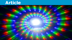
If one places a screen in the focal plane of the second spherical mirror while using a white light source, one will see a series of rainbows,  unlike a prism spectrometer, where there is only one rainbow.  Each of these rainbows is from a different order, e.g. ##m=-3,-2,-1,+1,+2,+3,… ##.  There is also the ##m=0 ## maximum, which is the white light image of the specular reflection of the entrance slit.  There will be some overlap in these rainbows. e.g. ## m \lambda=## 3(450)nm (violet)=2(675)nm (red), (the third order violet appears at the same location as the second order red), so that it is sometimes necessary to employ optical bandpass filters at the entrance slit to block light from unwanted portions of the spectrum that come from a different order ## m ##.  These filters are called order sorting filters.

Types of sources

Arc lamps of the elements such as hydrogen, helium, neon, krypton, sodium, and mercury have a number of  spectral lines from  electron transitions that can be readily observed.  Mercury also works very well for observing spectral line splittings that occur from the Zeeman effect, when the arc lamp is placed in a magnetic field, i.e. between the poles of a magnet.

See my next article: https://www.physicsforums.com/insights/fabry-perot-michelson-interferometry-fundamental-approach/

Comment Thread