
Higher Prequantum Geometry IV: The Covariant Phase Space – Transgressively
Show Complete Series
Part 1: Higher Prequantum Geometry I: The Need for Prequantum Geometry
Part 2: Higher Prequantum Geometry II: The Principle of Extremal Action – Comonadically
Part 3: Higher Prequantum Geometry III: The Global Action Functional — Cohomologically
Part 4: Higher Prequantum Geometry IV: The Covariant Phase Space – Transgressively
Part 5: Higher Prequantum Geometry V: The Local Observables – Lie Theoretically
Part 6: Examples of Prequantum Field Theories I: Gauge Fields
Part 7: Examples of Prequantum Field Theories II: Higher Gauge Fields
Part 8: Examples of Prequantum Field Theories III: Chern-Simons-type Theories
Part 9: Examples of Prequantum Field Theories IV: Wess-Zumino-Witten-type Theories
Part 10: Introduction to Perturbative Quantum Field Theory
The Euler-Lagrange ##p##-gerbes discussed in the previous article are singled out as being exactly the right coherent refinement of locally defined local Lagrangians that may be integrated over a ##(p+1)##-dimensional spacetime/worldvolume to produce a function, the action functional. In a corresponding manner, there are further refinements of locally defined Lagrangians by differential cocycles that are adapted to integration over submanifolds of ##\Sigma_{p+1}## of positive codimension. In codimension ##k## these will yield not functions, but ##p-k##-gerbes.
We consider this now for codimension 1 and find the covariant phase space of a locally variational field theory
equipped with its canonical (pre-)symplectic structure and equipped with a Kostant-Souriau prequantization of that.
As throughout, the following is indebted to discussion with Igor Khavkine.
First, consider the process of transgression in general codimension. In the convenient language of sheaves on smooth manifolds, it has the following simple incarnation.
Given a smooth manifold ##\Sigma##, then the mapping space ##[\Sigma,\mathbf{\Omega}^{p+1}]## into the smooth moduli space of ##(p+1)##-forms is the smooth space defined by the property that for any other smooth manifold ##U##, there is a natural identification
$$
\left\{
U \longrightarrow [\Sigma, \mathbf{\Omega}^{p+1}]
\right\}
\;\;
\simeq
\;\;
\Omega^{p+1}(U \times \Sigma)
$$
of smooth maps into the mapping space with smooth ##(p+1)##-forms on the product manifold ##U \times \Sigma##.
Now suppose that ##\Sigma = \Sigma_{p+1-k}## is a compact oriented smooth manifold of dimension ##p+1-k##. Then there is the fiber integration of differential forms on ##U \times \Sigma## over ##\Sigma## (e.g. [Bott-Tu]), which gives a map
$$
\int_{(U \times \Sigma_{p+1-k}) / U} : \Omega^{p+1}(U \times \Sigma_{p+1-k}) \longrightarrow \Omega^{k}(U)
\,.
$$
This map is natural in ##U##, meaning that it is compatible with the pullback of differential forms along with any smooth functions ##U_1 \to U_2##. This property is precisely what is summarized by saying that the fiber integration map constitutes a morphism in the sheaf topos
$$
\int_\Sigma : [\Sigma_{p+1-k}, \mathbf{\Omega}^{p+1}] \longrightarrow \mathbf{\Omega}^{k}
$$
This provides an elegant means to speak about transgression. Namely given a differential form ##\alpha \in \Omega^{p+1}(X)## (on any smooth space ##X##) modulated by a morphism ##\alpha : X \longrightarrow \mathbf{\Omega}##, then its transgression to the mapping space ##[\Sigma,X]## is simply the form in ##\Omega^{p+1-k}([\Sigma,X])## which is modulated by the composite
$$
\int_{\Sigma} [\Sigma, -]
\;:\;
[\Sigma,X]
\stackrel{[\Sigma,\alpha]}{\longrightarrow}
[\Sigma, \mathbf{\Omega}^{p+1}]
\stackrel{\int_{\Sigma}}{\longrightarrow}
\mathbf{\Omega}^{k}
$$
of the fiber integration map above with the image of ##\alpha## under the functor ##[\Sigma,-]## that forms mapping spaces out of ##\Sigma##.
All this works verbatim also in the context of PDEs over ##\Sigma##. For instance if ##L : E \longrightarrow \mathbf{\Omega}^{p+1}_H## is a local Lagrangian on (the jet bundle of) a field bundle ##E## over ##\Sigma_{p+1}## as before, then the action functional that it induces, as in the previous article, is the transgression to ##\Sigma_{p+1}##:
$$
S : [\Sigma,E]_\Sigma \stackrel{[\Sigma,L]_\Sigma}{\longrightarrow} [\Sigma, \mathbf{\Omega}^{p+1}_H]_\Sigma
\stackrel{\int_\Sigma}{\longrightarrow} \mathbf{\Omega}^0
\,.
$$
But now the point is that we have the analogous construction in higher codimension ##k##, where the Lagrangian does not
integrate to a function (a differential 0-form) but to a differential ##k##-form.
And all this goes along with passing from globally defined differential forms to Cech-Deligne cocycles.
For more background and more details see also the lecture notes at
- geometry of physics — differential forms
- geometry of physics — integration
To apply this for codimension ##k = 1##, consider now ##p##-dimensional submanifolds ##\Sigma_p \rightarrow \Sigma## of spacetime/worldvolume. Write ##N^\infty_\Sigma \Sigma_p## for the formal normal neighbourhood of ##\Sigma_p## in ##\Sigma##, i..e. the infinitesimal thickening of ##Sigma_p## inside ##\Sigma##. In practice one is often, but not necessarily, interested in ##\Sigma_p## being a Cauchy surface, which means that the induced restriction map
$$
[\Sigma_{p+1},\mathcal{E}]
\longrightarrow
[N^\infty_\Sigma \Sigma_p, \mathcal{E}]
$$
(from field configurations solving the equations of motion on all of ##\Sigma## to normal jets of solutions on ##\Sigma_p##) is an equivalence. An element in the solution space ##[\Sigma_{p+1},\mathcal{E}]## is a classical state of the physical system that is being described, a classical trajectory of a field configuration over all of spacetime. Its image in ##[N^\infty_\Sigma\Sigma_{p},\mathcal{E}]## is the restriction of that field configuration and of all its derivatives to ##\Sigma_p##.
In many — but not in all — examples of interest, classical trajectories are fixed once their first-order derivatives over a Cauchy surface are known. In these cases, the phase space may be identified with the cotangent bundle of the space of field configurations on the Cauchy surface
$$
[N^\infty_\Sigma \Sigma_p, \mathcal{E}]
\simeq
T^\ast [\Sigma_p, E]
\,.
$$
The expression on the right is often regarded as the definition of phase spaces. But since the equivalence with the left-hand side does not hold generally, we will not restrict attention to this simplified case and instead consider the solution space ##[\Sigma,\mathcal{E}]_\Sigma## as the phase space. To emphasize this more general point of view, one sometimes speaks of the
covariant phase space. Here “covariance” refers to invariance under the action of the diffeomorphism group of ##\Sigma##, meaning here that no space/time split in the form of a choice of Cauchy surface is made (or necessary) to define the phase space, even if a choice of Cauchy surface is possible and potentially useful for parameterizing phase space in terms of initial value data.
Since the notation ##[N^\infty_\Sigma \Sigma_p, \mathcal{E}]_\Sigma## is getting a bit heavy, from now on we will notationally suppress the denotation of the infinitesimal normals and just write
$$[\Sigma_p, \mathcal{E}]_\Sigma := [N^\infty_\Sigma \Sigma_p, \mathcal{E}]\,.$$
Since the only sensible interpretation of the left hand is the right hand, no confusion should arise.
It is crucial that the covariant phase space ##[\Sigma,\mathcal{E}]_\Sigma## comes equipped with further geometric structure which remembers that this is not just any old space, but the space of solutions of a locally variational differential equation. To see how this comes about, let us write ##(\mathbf{\Omega}^{p+1}_{\mathrm{cl}})_{\Sigma}## for the moduli space of all closed ##p+1##-forms on PDEs. This is to mean that if ##E## is a bundle over ##\Sigma##, and regarded as representing the space of solutions of the trivial PDE on sections of ##E##, then morphisms ##E \longrightarrow (\mathbf{\Omega}^{p+1})_{\Sigma}## are equivalent to closed differential ##(p+2)##-forms on the jet bundle of ##E##.
$$
\left\{
E \longrightarrow (\mathbf{\Omega}^{p+1})_\Sigma
\right\}
\;\;\simeq\;\;
\Omega^{p+1}_{\mathrm{cl}}(J^\infty_\Sigma E)
\,.
$$
The key now is that there is a natural filtration on these differential forms adapted to spacetime codimension. This is part of a bigrading structure on differential forms on jet bundles known as the variational bicomplex . In its low stages it looks as follows:
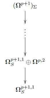
The lowest item here is what had concerned us in a previous article, it is the moduli of ##p+2##-forms which have ##p+1## of their legs along spacetime/worldvolume ##\Sigma## and whose remaining vertical leg along the space of local field configurations depends only on the field value itself, not on any of its derivatives. This was precisely the correct recipient of the variational curvature, hence the variational differential of horizontal ##(p+1)##-forms representing local Lagrangians.
But now that we are moving up in codimension, this coefficient will disappear, as these forms do not contribute when integrating just over ##p##-dimensional hypersurfaces. The correct coefficient for that case is instead clearly ##\mathbf{\Omega}^{p,2}##, the moduli space of those ##(p+2)##-forms on jet bundles which have ##p## of their legs along spacetime/worldvolume, and the remaining two along with the space of local field configurations. (There is a more abstract way to derive this filtration from first principles,
and which explains why we have restriction to “source forms” (not differentially depending on the jets),
indicated by the subscript, only in the bottom row. But for the moment we just take that little subtlety for granted.)
So ##\mathbf{\Omega}^{p,2}## is precisely the space of those ##(p+2)##-forms on the jet bundle that become (pre-)symplectic 2-forms on the space of field configurations once evaluated on a ##p##-dimensional spatial slice ##\Sigma_p## of spacetime ##\Sigma_{p+1}##. We may think of this as a current on spacetime with values in 2-forms on fields.
Indeed, there is a canonical such presymplectic current for every locally variational field theory [Zuckerman 87, Khavkine 14]. To see this, we ask for a lift of the purely horizontal locally defined Lagrangian ##L_i## through the variational bicomplex to a ##(p+1)##-form on the jet bundle whose curvature ##d(L_i + \Theta_i)## coincides with the Euler-Lagrange form ##\mathrm{EL} = \delta_V L_i## in vertical degree 1. Such a lift ##L_i + \Theta_i## is known as a Lepage form for ##L_i## (e.g. [GMS 09, 2.1.2]).
Notice that it is precisely the restriction to the shell ##\mathcal{E}## that makes the Euler-Lagrange form ##\mathrm{EL}_i## disappear, by construction, so that only the new curvature component ##\Omega_i## remains as the curvature of the Lepage form on the shell:
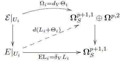
The condition means that the horizontal differential of ##\Theta_i## has to cancel against the horizontally exact part that appears when decomposing the differential of ##L_i## as discussed in a previous article. Hence, up to horizontal derivatives, this ##\Theta_i## is in fact uniquely fixed by ##L_i##:
$$
\begin{aligned}
d (L_i + \Theta_i) & = (\mathrm{EL}_i – d_H (\Theta_i + d_H(\cdots))) + (d_H \Theta_i + d_V \Theta_i)
\\
& = \mathrm{EL}_i + d_V \Theta_i
\\
& =: \mathrm{EL}_i + \Omega_i
\end{aligned}
\,.
$$
The new curvature component
$$
\Omega \in \Omega^{p,2}(J^\infty_\Sigma E)
$$
whose restriction to patches is given this way
$$
\Omega|_{U_i} := d_V \Theta_i
$$
is known as the presymplectic current [Zuckerman 87, Khavkine 14]. Because, by the way we found its existence, this is such that its transgression over a codimension-1 submanifold ##\Sigma_p \longrightarrow \Sigma## yields a closed 2-form (a “presymplectic 2-form”) on the covariant phase space:
$$
\omega := \int_{\Sigma_p} [\Sigma_p, \Omega]
\in
\Omega^2([\Sigma_p, \mathcal{E}])
\,.
$$
Since ##\Omega## is uniquely specified by the local Lagrangians ##L_i##, this gives the covariant phase space canonically the structure of a presymplectic space ##([\Sigma,\mathcal{E}], \omega)##, and this is just the structure on phase space that reflects the fact that the phase space arises as the solutions to a locally variational classical field theory. This is the reason why phase spaces in classical mechanics are given by (pre-)symplectic geometry as in [Arnold 89].
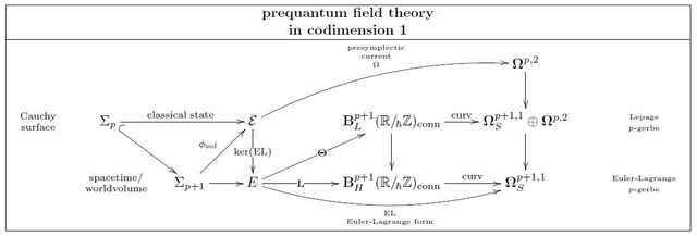
But by the discussion in the previous article, we do not just consider a locally variational field classical field theory to start with, but a prequantum field theory. Hence in fact there is more data before transgression than just the new curvature components ##d_V \Theta_i##, there is also Cech cocycle coherence data that glues the locally defined ##\Theta_i## to a globally consistent differential cocycle.
We write ##\mathbf{B}^{p+1}_L(\mathbb{R}/_{\!\hbar}\mathbb{Z})## for the moduli space for such coefficients (with the subscript for “Lepage”), so that morphisms ##E \longrightarrow \mathbf{B}^{p+1}_L(\mathbb{R}/_{\!\hbar}\mathbb{Z})##
are equivalent to properly prequantized globally defined Lepage lifts of Euler-Lagrange ##p##-gerbes.
In summary then, the refinement of an Euler-Lagrange ##p##-gerbe ##\mathbf{L}## to a Lepage-##p##-gerbe ##\Theta## is given by the following diagram:
And now higher prequantum geometry bears fruit: since transgression is a natural operation, and since the differential coefficients ##\mathbf{B}_H^{p+1}(\mathbb{R}/_{\!\hbar}\mathbb{Z})_{\mathrm{conn}}## and ##\mathbf{B}^{p+1}_L(\mathbb{R}/_{\!\hbar}\mathbb{Z})## precisely yield the coherence data to make the
local integrals over the locally defined differential forms ##L_i## and ##\Theta_i## be globally well defined, we may now hit this entire diagram with the transgression functor ##\int_{\Sigma_p} [\Sigma_p,-]## to obtain this diagram:
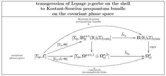
This exhibits the transgression
$$
\mathbf{\theta} := \int_{\Sigma_p} [\Sigma_p,\mathbf{\Theta}]
$$
of the Lepage ##p##-gerbe ##\mathbf{\Theta}## as a ##(\mathbb{R}/_{\!\hbar}\mathbb{Z})##-connection whose curvature is the canonical presymplectic form.
But this ##([\Sigma,\mathcal{E}]_\Sigma,\mathbf{\theta})## is just the structure that Souriau originally called and demanded as a prequantization of the (pre-)symplectic phase space ##([\Sigma,\mathcal{E}]_\Sigma,\omega)##. Conversely, we see that the Lepage ##p##-gerbe ##\mathbf{\Theta}## is a “de-transgression” of the Kostant-Souriau prequantization of covariant phase space in codimension-1 to a higher prequantization in full codimension. In particular, the higher prequantization constituted by the Lepage ##p## gerbe constitutes a compatible choice of Kostant-Souriau prequantizations of covariant phase space for all choices of codimension-1 hypersurfaces at once. This is a genuine reflection of the fundamental locality of the field theory, even if we look at the field configurations globally over all of a (spatial) hypersurface ##\Sigma_p##.
I am a researcher in the department Algebra, Geometry and Mathematical Physics of the Institute of Mathematics at the Czech Academy of the Sciences (CAS) in Prague.
Presently I am on leave at the Max Planck Institute for Mathematics in Bonn.


[QUOTE=”Urs Schreiber, post: 5267503, member: 567385″]No, that means that on sufficiently small neighbourhoods of field configurations there is a good supply of spacetime local and gauge invariant observables that are functions just of those field configurations in that small neighbourhood. For larger neighbourhoods no such observables will exist anymore, but the small neighbourhoods for which they do exist cover all of the (phase) space of fields.[/QUOTE]
Is the idea of “quantum similarity” from this (paper by Smolin) consistent with what is meant by “a small neighborhood of field configurations” that “covers all of the (phase) space of fields”?
I’m trying to understand if Khavkine is arguing against QM non-locality or for it – by saying that the local observables will have characteristics that are due to their special “multi-local” status in phase-space (which is what Smolin seemed to be saying).
[URL]http://arxiv.org/abs/1506.02938[/URL]
[SIZE=6][B]Quantum mechanics and the principle of maximal variety[/B][/SIZE]
[URL=’http://arxiv.org/find/quant-ph/1/au:+Smolin_L/0/1/0/all/0/1′]Lee Smolin[/URL]
(Submitted on 9 Jun 2015)
Quantum mechanics is derived from the principle that the universe contain as much variety as possible, in the sense of maximizing the distinctiveness of each subsystem.
The quantum state of a microscopic system is defined to correspond to an ensemble of subsystems of the universe with identical constituents and similar preparations and environments. A new kind of interaction is posited amongst such similar subsystems which acts to increase their distinctiveness, by extremizing the variety. In the limit of large numbers of similar subsystems this interaction is shown to give rise to Bohm’s quantum potential. As a result the probability distribution for the ensemble is governed by the Schroedinger equation.
The measurement problem is naturally and simply solved. Microscopic systems appear statistical because they are members of large ensembles of similar systems which interact non-locally. Macroscopic systems are unique, and are not members of any ensembles of similar systems. Consequently their collective coordinates may evolve deterministically.
This proposal could be tested by constructing quantum devices from entangled states of a modest number of quits which, by its combinatorial complexity, can be expected to have no natural copies.
Also, this quote from the paper I linked to in post #12 seemed relevant. p2.
[I]”Given this, the next problem is to identify observables that, in an appropriate sense, reduce to the local observables of field theory. A central idea here is that such observables should be “relational.” In classical general relativity, one approach is to discuss the spacetime location of events relative to some physical reference body, such as a clock on the earth. Specifying events in this way allows one to build relational classical observables, in an approach going back to [5], such as the value of RabcdRabcd at an event specified by its relation to the earth and to the time registered on the clock. Such quantities capture a certain sense of locality, but are nevertheless observables, in the sense that they define diffeomorphism-invariant functions on the space of classical solutions. The question then is how, and to what extent, similar correlations can be used to extract physical information in quantum gravity. The literature contains a number of approaches to this question, see e.g. [1,5-13]”[/I]
[QUOTE=”Jimster41, post: 5267173, member: 517770″]By “as a sheaf of functions on phase space” does that mean an observable would be spread out in space-time?[/QUOTE]
No, that means that on sufficiently small neighbourhoods of field configurations there is a good supply of spacetime local and gauge invariant observables that are functions just of those field configurations in that small neighbourhood. For larger neighbourhoods no such observables will exist anymore, but the small neighbourhoods for which they do exist cover all of the (phase) space of fields.
[QUOTE=”Urs Schreiber, post: 5254885, member: 567385″]A point that Igor Khavkine has been making for a while (for instance in [URL=’https://www.youtube.com/watch?v=G5O9RKmXyfM’]this talk[/URL]) is that the full power of available mathematical machinery for handling local field theories has rarely been fully applied, notably so in the case of effective gravity.
A striking example is the construction of local and gauge-invariant observables in gravity. Folk-lore held that these simply do not exist, a claim that leads to a wealth of apparent problems that are often claimed to necessitate speculative modifications of established physical principles. But a careful mathematical analysis shows that these observables do indeed exist, not as global functions, but as a sheaf of functions on phase space:
[LIST]
[*][URL=’http://ncatlab.org/nlab/show/Igor+Khavkine’]Igor Khavkine[/URL], [I]Local and gauge invariant observables in gravity[/I], Class. Quantum Grav. 32 185019, 2015 ([URL=’https://arxiv.org/abs/1503.03754′]arXiv:1503.03754[/URL], [URL=’http://cqgplus.com/2015/09/16/local-and-gauge-invariant-observables-in-gravity/’]CQG+[/URL], [URL=’http://www.science.unitn.it/~moretti/convegno/khavkine.pdf’]pdf slides[/URL] for talk at [URL=’http://www.science.unitn.it/~moretti/convegno/convegno.html’]Operator and Geometric Analysis on Quantum Theory[/URL] Levico Terme, Italy, September 2014)
[/LIST]
[/QUOTE]
By “as a sheaf of functions on phase space” does that mean an observable would be spread out in space-time?
If so does that mean distributed discretely, where some parts of the phase space don’t support those functions?
I found another paper that seems to be saying something like what Khavkine is saying.
[URL]http://arxiv.org/pdf/hep-th/0512200v4.pdf[/URL]
[SIZE=6][B]Observables in effective gravity[/B][/SIZE]
[URL=’http://arxiv.org/find/hep-th/1/au:+Giddings_S/0/1/0/all/0/1′]Steven B. Giddings[/URL], [URL=’http://arxiv.org/find/hep-th/1/au:+Marolf_D/0/1/0/all/0/1′]Donald Marolf[/URL], [URL=’http://arxiv.org/find/hep-th/1/au:+Hartle_J/0/1/0/all/0/1′]James B. Hartle[/URL]
(Submitted on 16 Dec 2005 ([URL=’http://arxiv.org/abs/hep-th/0512200v1′]v1[/URL]), last revised 8 Sep 2006 (this version, v4))
We address the construction and interpretation of diffeomorphism-invariant observables in a low-energy effective theory of quantum gravity. The observables we consider are constructed as integrals over the space of coordinates, in analogy to the construction of gauge-invariant observables in Yang-Mills theory via traces. As such, they are explicitly non-local. Nevertheless we describe how, in suitable quantum states and in a suitable limit, the familiar physics of local quantum field theory can be recovered from appropriate such observables, which we term `pseudo-local.’ We consider measurement of pseudo-local observables, and describe how such measurements are limited by both quantum effects and gravitational interactions. These limitations support suggestions that theories of quantum gravity associated with finite regions of spacetime contain far fewer degrees of freedom than do local field theories.
[quote=”Urs Schreiber, post: 5254769″][QUOTE=”David Corfield, post: 5253853, member: 573332″]There are some (three?) occasions where the Latex didn’t compile. And some typos: …[/QUOTE]
Thanks! Fixed now.
[QUOTE=”David Corfield, post: 5253853, member: 573332″]I wonder how much these constructions are arising through abstract general considerations. [/QUOTE]
Everything! For the present series I am downplaying the general abstract perspective, clearly, but everything I am saying here flows naturally out of differentially cohesive homotopy theory. The key point is that the variational bicomplex is locally equivalent to the de Rham complex. This means that as we start with ordinary differential cohomology in the base differentially cohesive infinity-topos and then send that to the topos of PDEs, there a “finer Poincare lemma” appears which allows to resolve the constant real coefficients by a chain complex adapted to the horizontal stratification. This way the variational Euler-differential appears all by itself as the curvature of those “Euler-Lagrange p-gerbes”. Anyway, I should talk about this in more detail later.
[QUOTE=”David Corfield, post: 5253853, member: 573332″]And how much (presumably less) in the realm of arithmetic jet spaces?[/QUOTE]
One has to beware that the [URL=’http://ncatlab.org/nlab/show/arithmetic%20jet%20space’]arithmetic jet spaces[/URL] of Buium do not capture the general concept of jets. I think the right way to put it is that for ##X## an arithmetic scheme, then Buium’s arithmetic jet space is to be thought of as the jets of the bundle ## X times mathrm{Spec}(mathbb{Z}) to mathrm{Spec}(mathbb{Z}) ##. More generally one need jet bundles of more general arithmetic bundles.[/quote]”More generally one need jet bundles of more general arithmetic bundles.”
Is he as limited as this? In ‘Differential calculus with integers’ (http://arxiv.org/abs/1308.5194) he’s talking about taking jet spaces of spec(W(R)) (p-typical Witt vectors of R) in section 1.2.12.
And problem 3.1 states:
“Study the arithmetic jet spaces Jn(X) of curves X (and more general varieties) with bad reduction.”
Many of the constructions appearing in these posts appear there, e.g., variational complex, Euler-Lagrange total differential form and Noether’s theorem appear in 1.2.9. But maybe just as exposition.
It seems it’s his ‘Arithmetic Differential Equations’ where one sees his “arithmetic” Euler-Lagrange operators and Noether’s theorem (p. 98 of https://books.google.co.uk/books?id=aqwYKFjW5nwC). It’s not so easy to find out the breadth of jet spaces treated there.
[QUOTE=”Shyan, post: 5254606, member: 160907″]I know Arnold’s text, but the book I plan to read about more theoretical aspects of classical mechanics is “Mechanics: From Newton’s Laws to Deterministic Chaos” by Florian Scheck. Is it more or less equivalent to Arnold’s?[/QUOTE]
His ambition is there, to be at the same level, but his presentation is not something I like. He starts at the average level of Marion/Thornton for about 330 pages, then turns the mathematics on what he already wrote about.
[QUOTE=”David Corfield, post: 5254865, member: 573332″] Would it be fair to say this work hasn’t been exploited by the community as much as it might have been?[/QUOTE]
A point that Igor Khavkine has been making for a while (for instance in [URL=’https://www.youtube.com/watch?v=G5O9RKmXyfM’]this talk[/URL]) is that the full power of available mathematical machinery for handling local field theories has rarely been fully applied, notably so in the case of effective gravity.
A striking example is the construction of local and gauge-invariant observables in gravity. Folk-lore held that these simply do not exist, a claim that leads to a wealth of apparent problems that are often claimed to necessitate speculative modifications of established physical principles. But a careful mathematical analysis shows that these observables do indeed exist, not as global functions, but as a sheaf of functions on phase space:
[LIST]
[*][URL=’http://ncatlab.org/nlab/show/Igor+Khavkine’]Igor Khavkine[/URL], [I]Local and gauge invariant observables in gravity[/I], Class. Quantum Grav. 32 185019, 2015 ([URL=’https://arxiv.org/abs/1503.03754′]arXiv:1503.03754[/URL], [URL=’http://cqgplus.com/2015/09/16/local-and-gauge-invariant-observables-in-gravity/’]CQG+[/URL], [URL=’http://www.science.unitn.it/~moretti/convegno/khavkine.pdf’]pdf slides[/URL] for talk at [URL=’http://www.science.unitn.it/~moretti/convegno/convegno.html’]Operator and Geometric Analysis on Quantum Theory[/URL] Levico Terme, Italy, September 2014)
[/LIST]
[QUOTE=”Shyan, post: 5253607, member: 160907″]
So what branches of Mathematics do I need to learn? I think they are algebraic topology and algebraic geometry (and category theory?), are they?
Thanks[/QUOTE]
I am rather freely speaking category theory here, that’s true. But for the moment all the series is really referring to is the concept of presheaf and the [URL=’http://ncatlab.org/nlab/show/Yoneda+lemma’]Yoneda lemma[/URL]. Under the hood the Beck monadicity theorem is playing a key role, but just to follow the story you don’t need that.
And then of algebraic topology the series presently needs mainly the concept of sheaf hypercohomology in its presentation by Cech cohomology. I have been writing lecture notes that gradually introduce precisely the material that I am using here at
[LIST]
[*][B][URL=’http://ncatlab.org/nlab/show/geometry+of+physics’]nLab: geometry of physics[/URL][/B]
[/LIST]
These notes consist of a list of sub-pages that have detailed exposition and introduction to the various subjects needed, complete with further pointers to the literature.
Essentially this same lecture series is also available in pdf format, as section 1.2 of
[LIST]
[*][URL=’https://dl.dropboxusercontent.com/u/12630719/dcct.pdf’][B]Differential cohomology in a cohesive topos[/B][/URL]
[/LIST]
(just focus on section 1).
[QUOTE=”David Corfield, post: 5253853, member: 573332″]There are some (three?) occasions where the Latex didn’t compile. And some typos: …[/QUOTE]
Thanks! Fixed now.
[QUOTE=”David Corfield, post: 5253853, member: 573332″]I wonder how much these constructions are arising through abstract general considerations. [/QUOTE]
Everything! For the present series I am downplaying the general abstract perspective, clearly, but everything I am saying here flows naturally out of differentially cohesive homotopy theory. The key point is that the variational bicomplex is locally equivalent to the de Rham complex. This means that as we start with ordinary differential cohomology in the base differentially cohesive infinity-topos and then send that to the topos of PDEs, there a “finer Poincare lemma” appears which allows to resolve the constant real coefficients by a chain complex adapted to the horizontal stratification. This way the variational Euler-differential appears all by itself as the curvature of those “Euler-Lagrange p-gerbes”. Anyway, I should talk about this in more detail later.
[QUOTE=”David Corfield, post: 5253853, member: 573332″]And how much (presumably less) in the realm of arithmetic jet spaces?[/QUOTE]
One has to beware that the [URL=’http://ncatlab.org/nlab/show/arithmetic%20jet%20space’]arithmetic jet spaces[/URL] of Buium do not capture the general concept of jets. I think the right way to put it is that for ##X## an arithmetic scheme, then Buium’s arithmetic jet space is to be thought of as the jets of the bundle ## X times mathrm{Spec}(mathbb{Z}) to mathrm{Spec}(mathbb{Z}) ##. More generally one need jet bundles of more general arithmetic bundles.
[QUOTE=”dextercioby, post: 5254346, member: 1064″]This is the highest level tutorial ever posted on PF. High level differential geometry, diff. and algebraic topology. To reach this level of maths knowledge, you need to start early. Did you read Arnold’s mechanics text ?[/QUOTE]
I know Arnold’s text, but the book I plan to read about more theoretical aspects of classical mechanics is “Mechanics: From Newton’s Laws to Deterministic Chaos” by Florian Scheck. Is it more or less equivalent to Arnold’s?
[QUOTE=”Shyan, post: 5253607, member: 160907″]I don’t know whether this is a proper question to ask here or not, but I can’t resist any more.
This whole series is way above my head but I somehow understand its importance and beauty, so I’m eager to learn it, actually adding it to my list of to-learn things!
So what branches of Mathematics do I need to learn?
I think they are algebraic topology and algebraic geometry (and category theory?), are they?
Thanks[/QUOTE]
This is the highest level tutorial ever posted on PF. High level differential geometry, diff. and algebraic topology. To reach this level of maths knowledge, you need to start early. Did you read Arnold’s mechanics text ?
I don’t know whether this is a proper question to ask here or not, but I can’t resist any more.
This whole series is way above my head but I somehow understand its importance and beauty, so I’m eager to learn it, actually adding it to my list of to-learn things!
So what branches of Mathematics do I need to learn?
I think they are algebraic topology and algebraic geometry (and category theory?), are they?
Thanks
Thanks. I see Anderson has a G-equivariant version for some group of symmetries of E, which delivers a G-invariant Euler-Lagrange complex.He paints a picture of an ambitious research program. Would it be fair to say this work hasn't been exploited by the community as much as it might have been?
There are some (three?) occasions where the Latex didn't compile.And some typos: bunle; invariace; codimenion; depeningThis post will need some re-reading on my part. I wonder how much these constructions are arising through abstract general considerations. E.g. where one to want such a thing, would they go through in the complex analytic realm? And how much (presumably less) in the realm of arithmetic jet spaces?