
Introduction to Electric Vector Potential and Its Applications
Main Point: The electric vector potential offers a means of determining the non-conservative component of mixed stationary or quasi-stationary electric field
While many are familiar with the static magnetic vector potential
## \bf A = (\mu/4\pi) \int \bf j~ dv/s ##
with ## \bf j ## = current (area) density within differential volume ## dv ## and ## s ## = distance from ## dv ## to the point of observation, the magnetic field is then derivable from
## \bf B = \nabla \times \bf A ##.
However, finite vector potentials exist in any vector field ## F ## for which ## \nabla \times \bf F \neq 0 ##. If the field is wholly scalar the vector potential is zero.
The Helmholtz decomposition theorem can be reduced for any electric field to stating that there are two kinds of E field, one for which ## \nabla \times \bf E = 0 ## (a “scalar” field ## E_s ##), and the other for which ## \nabla \times \bf E \neq 0 ##, a non-conservative field ## E_m ##. An E field can comprise both kinds of field and we call that a mixed field: ## \bf E = \bf E_m + \bf E_s ##.
The vector potential can serve as a means of identifying the ## \bf E_m ## part of any static or quasi-static mixed E field at any observation point. By doing so it ipso facto identifies both the irrotational and non-conservative components at that point.
In fact, a good name for the electric vector potential is “## E_m ## detector.”
The generalized vector potential for a stationary or quasi-stationary field ## \bf F ## obeys
## \bf F = -\nabla U + \nabla \times \bf W ##
where the scalar potential is ## U ## and the vector potential is ## \bf W ##.
We also know from mathematics that
## \nabla^2 \bf W = -\nabla (\nabla \cdot \bf W)~ – \nabla \times (\nabla \times \bf W) ##
For our vector potential ## \bf W ## we are however free to choose ## \nabla \cdot \bf W = 0 ## (by gage invariance or direct verification). Then
## -\nabla^2 \bf W = \nabla \times \bf F ##
which are of course 3 scalar equations, one of which is
## -(\nabla^2 W)_z = (\nabla \times \bf F)_z ##
and by similarity to the known expression for scalar electric potential
## U = (1/4\pi) \int \rho/\epsilon~ dv/s ##
if we replace ## \rho / \epsilon ## with ## (\nabla \times \bf W)_z ##
we obtain the general relation for a vector field ## \bf F ## with vector potential ## \bf W ## as
## \bf W = (1/4\pi) \int (\nabla \times \bf F)~ dv/s. ##
and ## \bf F = \nabla \times \bf W – \nabla U ##.
But for an electromagnetic E field we also know that ## \nabla \times \bf E = -\partial \bf B/\partial t ## so we have the electric vector potential ## \bf W ##:
$$ \bf W = (1/4\pi) \int (-\partial \bf B/\partial t) ~dv/s $$,
with ## \bf E_m = \nabla \times \bf W ## and ## \bf E_s = -\nabla U ##.
As a simple example let us apply this formula to a circular B field of infinite length ## -\infty < z < +\infty ##, cross-sectional area ##a## so flux ##\phi = aB ##. . We seek the E field outside the B field. We then all know a priori that in cylindrical coordinates
## \bf E = -(\partial \phi/\partial t)/2\pi~ r ~ \hat {\bf \theta} ##
forming circles of radii r.
By the electric vector potential on the other hand,
## \bf W = (1/4\pi) \int (\nabla \times \bf E)~dv/s ##
## = -(1/4\pi) \dot B\int dv/s. ##
We have ## dv = a ~dz ##
## \phi = aB ##
## s = (z^2 + r^2)^{1/2} ##, so
## \bf W = W_z \hat {\bf k} ## since ## \bf W ## is in the direction of ## \bf B ##
## W_z(r,d) =~ – (1/4\pi) \dot \phi \int_{-d}^d ~ dz/(z^2 +r^2)^{1/2} ##
## W_z(r,d) = ~ – (1/4\pi) \dot \phi ~~ \ln~ \frac {(z^2 + r^2)^{1/2} + z} {(z^2 + r^2)^{1/2} – z} ## evaluated (z= d) – (z= – d).
Now ## \bf E = \nabla \times \bf W ## or
## E_{\theta} = lim ~ d \to \infty ## of ## \partial {W_z(r,d)}/\partial r ##
## =~ – (1/4\pi) \dot \phi ~~ lim ~~d \to \infty of 2d/r(r^2+ d^2)^{1/2} ##
## = ~- \dot \phi/2\pi~r ##
i.e. the answer we knew beforehand.
****************************************************************************
Now, to some folks’ annoyance, I will again put a resistive ring concentric with a time-varying B field of infinite extent at radius ## a ##. Assume first a uniform ring of resistance ## r ##. The formula gives the same answer as without the ring: ## E_m = -\partial \phi/\partial t/2\pi a ## all around the ring.
Now assume half the ring has resistance ## r ## and the other half ## 2r ##. See fig. 1:
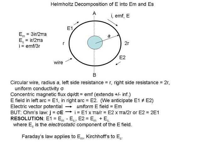
Fig. 1 Non-uniform resistive ring surrounding time-varying B field
The electric vector potential formula still gives the same answer ## E_m ##, as it should.
But, but – we can readily determine via Faraday’s and Ohm’s laws that the ## r ## side has half the E field of the ## 2r ## side. What gives?
The truth, inconvenient though it may be, is in my last blog: the fields are a mixture of scalar and non-conservative fields.
The electric vector potential finds only the part of the E field ascribable directly to the time-varying B field, in other words the ##E_m ## part. (The electrostatic part ## E_s ## is of course ## -\nabla U ## for the two equal & opposite ## E_s ## fields.
Cf.
https://www.physicsforums.com/threads/how-to-recognize-split-electric-fields-comments.984872/
Now, one may wonder why bother with identifying split fields when most measurable parameters (voltmeter readings, joule heating, current, net E field, plus obeyance to Faraday’s law etc.) can all be found by assuming just one kind of E field?
My answer is twofold:
(a) the E fields inside and outside the ring are greatly affected by the free charges setting up the ## E_s ## fields. In Fig. 1, net positive free charge accumulates at A with an equal negative charge at B. (With the uniform ring there are no free charges, thus no impact on the fields. It’s just the same ## E_m ## as if there were no ring, with ## E_s = 0 ##.)
These field changes are not appreciable without an understanding of split fields.
(b) are we physicists or technicians? Do we want to know what’s really going on or not?
I am reminded of the ring laser gyro: the true explanation for the phase shift as a function of rotation rate can only be provided by relativity, i.e. the Sagnac effect. Yet we get exactly the same phase shift by ignoring relativity altogether, by simply adding the speed of rotation to the speed of light, Galilean style. So should we ignore the Sagnac effect and relativity?
Final note: the electric vector potential is more powerful than the faraday rule ## \oint \bf E \cdot \bf {dl} = – \partial \phi/\partial t ## since the faraday formula does not distinguish between electrostatic and emf-generated E fields, while the vector potential gives a point-by-point accurate reading for the emf part of the field around any closed loop. The rest must be electrostatic, by Helmholtz.
http://farside.ph.utexas.edu/teaching/em/lectures/node37.html
AB Engineering and Applied Physics
MSEE
Aerospace electronics career
Used to hike; classical music, esp. contemporary; Agatha Christie mysteries.


Electrostatics is a subset of electromagnetics. If it is valid for the general case of electromagnetics then obviously it also applies for the specific electrostatic case of a battery.
Anyway, since you are merely going to persist in the same misinformation as always we are done.
My blog and derivation of ## \bf W = (1/4\pi) \int (-\partial \bf B/|\partial t~ dv/s. ## was specifically for electromagnetic fields, as I emphasized.
However, my derivation, ## \bf W = (1/4\pi) \int (\nabla \times \bf F)~ dv/s. ## applies to all Em fields. – in fact, to all E fields since the elecrtic vector potential for the Es part = 0.
As I've tried to tell you may times, Em fields, and therefore electric vector potentials, are not limited to electromagnetic fields.
I gave several examples of the existence of Em fields in other cases, e.g. in a Seebeck-effect wire and a chemical battery. In the latter you of course took occasion to suggest Stanford Professor H H Skilling's text as "making the same mistake I made" after admitting it was "concerning" to you.
You might look at Prof. Skilling's biography . https://ethw.org/Hugh_H._Skilling.
Are you and @vanhees61 really that much wiser than he?
Sure, there is. It is very clear. You fixed it with this equation which you posted in your current blog:
Congratulations for finally getting it right, that is good to see.
Now, for any static situation, like the battery example, we have ##\partial \mathbf B/\partial t =0## by definition of static. Therefore by your own correct equation posted here ##\mathbf W = 0##. So ##\nabla \times \mathbf W = 0## and therefore ##E_m=0##, which is in clear contradiction to your previous incorrect claims that I tried unsuccessfully to point out to you previously.
As I pointed out, many times, in my blog.
Retarded fields have nothing whatever to do with electrostatic/magnetostatic fields, which is why I couldn't figure out why you went on & on about it.
… which is the problem I mentioned ...
The split E field is E = Em + Es.
Em obey Maxwell, Es obey Kirchhoff.
So a split E field does obey the Em part of it.
Must I repeat this, over & over again?
Some morning while you're enjoying your coffee and Speckpfannkuchen, perhaps you might think about the following:
You have a solenoid with zero-resistance wiring (as depicted in Feynman's Vol II chapt. 22 sect. 22.1 & Fig. 22-1) A time-varying current runs through the wire, perhaps a di/dt = constant ramp.
There is therefore zero net E field in the wire, and a B flux ϕ inside the wire coils.
But – what happened to Faraday's ∮E⋅dl=−∂ϕ/∂t ? What happened to farady's E field? Or does Maxwell not apply to the E field in the wire?
Enjoy your breakfast.
Wrong. Es fields do obey Maxwell's equations.
All E foelds, Em or Es or any combination thereof, obey Maxwell's equations.
EDIT: I had a power interruption so I had no time to edit this statement. See below for what obeys Em and what obeys Es.
There was never any "major inconsistency" in my math. That is a figure of your vivid imagination.
There was never any "fix" needed.
You are of course free to rehash your "proof" from the comments section of my previous blog, which you chose to cut.
Yes – electrical engineers often use vector potentials for electric fields to solve certain types of dynamic (wave) problems. The problems I am referring to are those for which we apply equivalence principles to replace physical sources inside of a volume with fictional electric and magnetic currents on the surface of that volume that create the same fields in the region of interest. An electric vector potential is a convenient intermediate quantity when computing the fields from the (fictional) magnetic surface-currents, in exactly the same way that the 'regular' vector potential us useful for for computing fields from electric currents . Standard engineering electromagnetics texts use this approach, including the classic Time-Harmonic Electromagnetic Fields by Harrington. There are also a number of examples in the literature; one of the early ones is a 1939 Physical Review paper by Schelkunoff ("On diffraction and radiation of electromagnetic waves").
This application of the vector potential for electric fields is of course very different than described in the Insight article. I will let the rest of you argue about that!
Jason
They are not so much mathematical now, but previously they were big mathematical problems. I am glad to see that he fixed the major mathematical problems, and I am personally disinclined to argue the physics. Since the split fields don't obey Maxwell's equations on their own I see little physics value, but the Helmholtz decomposition is valid, so he is free to use it if he likes.
I am surprised to see this somewhat antagonistic invitation to participate. Since you had clearly and quietly fixed the severe mathematical problem that I previously pointed out, I thought that you wanted to go about quietly pretending that it had never happened. I was OK with that, leave the past in the past and all. So I am unsure why you would explicitly and antagonistically encourage my participation; I was content to allow you to quietly fix past mistakes and move on.
Did you want me to address your remaining minor mathematical mistakes? (I was not intending to but I certainly can). Or did you want me to come in ranting against your rather bombastically stated personal opinions and editorial comments? (I won't do that, you are entitled to have your opinions even if my opinion differs). Did you want an explicit confirmation from me that you have fixed your major mistake? (I can do that too, although since you were quiet about the fix I thought you didn't want to draw attention to it).
I think I was pretty clear about it. The problem was your major mathematical inconsistency, which I am glad to see you have fixed here. Although the fact that you have fixed the problem apparently without figuring out the problem makes me wonder if you did it accidentally and don't even recognize the important change that you have made.
Do you realize that what you say here is inconsistent with what you said previously? That is certainly not an issue, since it is always good to learn from past mistakes and improve. But then why would you claim to not have figured out the problem?
I expect the usual detractors with their irrelevant blatherings – one so far anyway, that I fully expected and that I actually welcomed as a sort of "old friend" – sort of! I expect one or two other usuals before the dust has settled. I can't figure out what their problem is. They have already dissed two texts by eminent physicists I have sent them copies of supporting the split E field view.
Otherwise, all quiet on the front so far.
Here's the course segment I ran across & got me thinking that an electric vector potential for static or quasi-static fields might be worth exploring. I actually was quite excited about it In fact I'm glad you asked for it as I will append it to my blog as a refrerence – should have in the first place.
The author develops the general vector potential as I have done (in abbreviated form) and relates it to the Maxwell equations. I think it's exciting reading.
http://farside.ph.utexas.edu/teaching/em/lectures/node37.html
The standard derivation (using the most simple case of "microscopic classical electrodynamics", i.e., the vacuum equations taking into account all charges and currents explicitly) is as follows. One starts from the homogeneous Maxwell equations (using Heaviside Lorentz units)
$$\vec{\nabla} \times \vec{E}+\frac{1}{c} \partial_t \vec{B}=0, \quad \vec{\nabla} \cdot \vec{B}=0.$$
From Helmholtz's decomposition theorem from the 2nd equation it follows that there is a vector potential such that
$$\vec{B}=\vec{\nabla} \times \vec{A}.$$
It's immediately clear that for the given magnetic field, ##\vec{A}## is only determined up to a gradient field of an arbitrary scalar field, i.e., the vector potential
$$\vec{A}'=\vec{A}-\vec{\nabla} \chi$$
for any scalar field ##\chi## discribes the same physics (gauge invariance).
Plugging this into the first equation, leads to
$$\vec{\nabla} \times (\vec{E}+1/c \partial_t \vec{A})=0,$$
and from Helmholtz's theorem this implies the existence of a scalar potential for the quantitiy in parantheses:
$$\vec{E}+\frac{1}{c} \partial_t \vec{A} = -\vec{\nabla} \Phi$$
or
$$\vec{E}=-\vec{\nabla} \Phi – \frac{1}{c} \partial_t \vec{A}.$$
Under the gauge transformation you have to also adapt this scalar potential
$$\vec{A}'=\vec{A}-\vec{\nabla} \chi \; \Rightarrow\; \Phi'=\Phi+\frac{1}{c} \partial_t \chi.$$
Indeed then
$$-\vec{\nabla} \Phi'-\frac{1}{c} \partial_t \vec{A}'=-\vec{\nabla} \Phi-\frac{1}{c} \partial_t \vec{A}=0.$$
The potentials then obey equations, derived from the inhomogeneous Maxwell equations, which however are gauge invariant and thus determine the potentials only up to a gauge transformation, and thus to make the solutions unique one has to impose a gauge constraint, fixing (or at least partially fixing) the gauge. Usual choices are the Lorenz gauge,
$$\vec{\nabla} \cdot \vec{A}+\frac{1}{c} \partial_t \Phi=0$$
and the Coulomb gauge
$$\vec{\nabla} \cdot \vec{A}=0.$$
This demonstrates that any split of the electromagnetic field components based on pieces of the expressions in terms of the potentials is not gauge invariant and thus physically not easy to interpret.
It is utmost important to stress that the direct application of Helmholtz's decomposition theorem to the potentials is not very convenient but one should rather use the retarded propgator of the d'Alembert operator (Lorenz gauge) and the Green's function of the Laplace operator (for the scalar potential in the Coulomb gauge). The use of the Helmholtz's decomposition theorem in the way shown in this Insights article is overly complicated leading to nonlocal descriptions of the fields. The final solution in terms of the retarded propagator for the fields (the socalled Jefimenko equations) which is the unique solution of the Maxwell equations in terms of the physical sources of the electromagnetic fields, which are the charge-current distributions and not some non-local integrals shown in the article, though they may be formally correct from a purely mathematical point of view.
The introduction of a vector potential for the electric field or a scalar potential for the magnetic field can be sometimes for calculations in special cases (though I'm not aware of the use of a vector potential for the electric field in the literature).