Massive Meets Massless: Compton Scattering Revisited
Table of Contents
Introduction
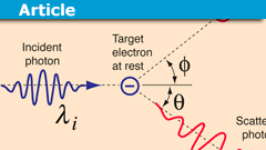
In a previous article entitled “Alternate Approach to 2D Collisions” we analyzed collisions between a moving and stationary object by defining the co-ordinate axes as being respectively parallel and perpendicular to the post-collision direction of motion of the stationary object. In this article, we will be adopting the same approach to analyze the well known physical phenomenon known as Compton scattering in which a photon collides with a stationary electron, imparts momentum to the latter, and hence loses momentum and energy which manifests in a change of direction (‘scattering’ angle) and wavelength (of the photon).
The established physics of Compton scattering relates the scattering angle (angle of deflection) to the change in wavelength of the incident photon according to the following expression: $$1-\cos\theta_d=\frac{\lambda_r-\lambda_i}{\lambda_c}=\frac{\Delta\lambda}{\lambda_c},$$ where ##\lambda_i## is the wavelength of the ‘incident’ photon , ##\lambda_r## the wavelength of the scattered or ‘refracted’ photon and ##\lambda_c## is the electron’s Compton Wavelength ##\frac{h}{m_ec}##. If we substitute ##\lambda_i=hc/E_i## , ##\lambda_r=hc/E_r## and ##\lambda_c=h/m_ec## where ##E_i## and ##E_r## are the energies of the incident and scattered photon respectively, we obtain the formula in energy form: $$1-\cos\theta=m_ec^2\left(\frac{1}{E_r}-\frac{1}{E_i}\right)=\frac{E_0\Delta E}{E_iE_r},$$ where ##E_o=m_ec^2## is the rest mass of the electron.
We aim to explore the scattering formula in both its wavelength and energy forms as well as introduce expressions for (the tan of) incident (pre-collision) and refracted (post-collision) angles of the photon. These angles are measured with reference to the normal – that is the line perpendicular to the direction of motion of the recoiling electron. They relate to the traditional scattering angle ##\theta_d ## according to the formula ##\theta_d=\theta_i-\theta_r##. Our notation will refer to the wavelength of the ‘incident’ photon as being ##\lambda_i## and the wavelength of the refracted (scattered) photon as being ##\lambda_r##. A similar notation will apply to frequencies and energies where applicable.
Classical Compton Scattering
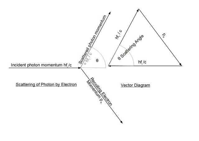
We begin with a pair of diagrams that essentially replicate those in Compton’s original paper. At left is a representation of the scattering process and to the right a vector diagram representing conservation of momentum for the same event:
We quote the basic theory more or less verbatim from Compton’s paper (albeit using the notation ##f_i## and ##f_r## in place of Compton’s original ##\nu_0## and ##\nu_\theta##):
Imagine as in the figure (at left) that an X-ray photon of frequency ##f_i## is scattered by an electron of mass ##m_e##. The momentum of the incident ray will be ##\frac{hf_i}{c}##, where c is the velocity of light and h is Planck’s constant, and that of the scattered ray ##\frac{hf_r}{c}## at an angle ##\theta## with the initial momentum. The principle of conservation of momentum accordingly demands that the momentum of recoil of the scattering electron shall equal the vector difference between the momenta of these two rays as in the figure (at right).
Compton wrote down the following two equations arising from conservation of momentum and conservation of energy respectively: $${\left(\frac{m_e\beta c}{\sqrt{(1-\beta^2)}}\right)}^2={\left(\frac{hf_i}{c}\right)}^2+{\left(\frac{hf_r}{c}\right)}^2-\frac{2h^2f_if_r\cos\theta}{c^2},$$
where ##\beta## is the ratio of the velocity of recoil of the electron to the velocity of light. But the energy ##hf_r## in the scattered quantum is equal to that of the incident quantum ##hf_i## less the kinetic energy of recoil of the scattering electron, ie: $$hf_r=hf_i-m_ec^2\left(\frac{1}{\sqrt{(1-\beta^2})}-1\right).$$
He went on to solve the simultaneous equations for the variables ##\beta## and ##f_r##.
In light of more recent developments favouring the use of energy (rather than wavelength) based equations, the route we will follow is to ‘convert’ the momentum equation into energy form by multiplying through by ##c^2## and making the following substitutions: $$E_i=hf_i \text{ , } E_r=hf_r\text{ and } {p_e}^2={\left(\frac{m_e\beta c}{\sqrt{(1-\beta^2)}}\right)}^2.$$Hence we obtain: $$(p_ec)^2={E_i}^2+{E_r}^2-2E_iE_r\cos\theta_d……Eqn\;1.$$ Since final electron energy is given by the standard expression ##E=\sqrt{{(p_ec)}^2+{E_0}^2}## where ##E_0=m_ec^2##, we may write: $${(p_ec)}^2=E^2-{E_0}^2=(E_0+(E_i-E_r))^2-{E_0}^2=2E_0(E_i-E_r)+(E_i-E_r)^2…Eqn\;2.$$From Eqn 1 and Eqn 2, PF user Vela provides us with some elegant algebra leading to an expression for scattering angle ##\theta_d##: $${E_i}^2+{E_r}^2-2E_iE_r\cos\theta_d=2E_0(E_i-E_r)+(E_i-E_r)^2$$ $$⇒{({E_i}-{E_r})}^2+2E_iE_r(1-\cos\theta_d)=2E_0(E_i-E_r)+(E_i-E_r)^2$$ $$⇒2E_iE_r(1-\cos\theta_d)=2E_0(E_i-E_r)$$ $$⇒1-\cos\theta_d=\frac{E_0\Delta E}{E_iE_r}=E_0\left(\frac{1}{E_r}-\frac{1}{E_i}\right).$$ The final result is the Compton scattering equation in energy form.
Historical Background
PF user JT Bell provides us with some historical background in respect of the development from a wavelength based to an energy-based equation for Compton scattering:
Introductory textbooks often give the Compton scattering equation in terms of wavelength ##\lambda## $$\lambda^\prime – \lambda = \frac h {mc} \left( 1 – \cos \theta \right).$$ I think this is because historically, a century ago, the relevant experiments used X-rays which were analyzed using diffraction through crystals (Bragg diffraction).
But nowadays, students are probably more likely to study Compton scattering experimentally using gamma-rays from commercial sources, and gamma detectors, for which energy in MeV is the natural unit. For many years, I taught a second-year undergraduate lab along these lines, using the energy-based version of the Compton scattering equation: $$\frac 1 {E^\prime} – \frac 1 E = \frac 1 {mc^2} \left( 1 – \cos \theta \right),$$ where both E’s and ##mc^2## are in MeV (or other energy-units).
Modern Physics Perspective
Since the author does not have the relevant expertise, the following derivation of the Compton scattering equation is kindly provided by PF user Vanhees71:
We analyse the kinematics of scattering of a massless particle with a massive particle. As usual in relativistic scattering the four-vector formalism is most convenient. We work in the “lab frame”, i.e., a photon hits an electron at rest. Thus
$$p_1=(p_{\gamma},p_{\gamma},0,0), \quad p_2=(m c,0,0,0).$$
Then (from energy and momentum conservation)
$$p_1’=(p_{\gamma}’,p_{\gamma}’ \cos \vartheta,p_{\gamma}’ \sin \vartheta,0), \quad p_2’=(m c-p_{\gamma}’,p_{\gamma}-p_{\gamma}’ \cos \vartheta,-p_{\gamma}’ \sin \vartheta).$$
To get ##p_{\gamma}’## we use the on-shell condition for the electron in the outgoing state, i.e.,
$$p_2^{\prime 2}=m^2 c^2=(p_1+p_2-p_1′)=(p_1-p_1′)^2 + 2 (p_1-p_1′) \cdot p_2 + m^2 c^2.$$
Multiplying out the Minkowski products and simplifying leads to
$$m c (p_{\gamma}-p_{\gamma}’)=p_{\gamma} p_{\gamma}’ (1-\cos \vartheta).$$
Dividing by ##p_{\gamma} p_{\gamma}’## and using the de Broglie wavelengths of the photon before and after the scattering as well as the compton wavelength of the electron ##m c =2 \pi \hbar/\lambda_{\text{Comp}}## one finds the well-known formula
$$\lambda’=\lambda + \lambda_{\text{Comp}} (1-\cos \vartheta).$$
or $$ 1-\cos \vartheta=m_ec^2\left(\frac{1}{E’}-\frac{1}{E}\right).$$ (author’s addition).
Incident and Refracted Angles
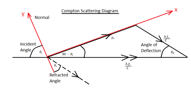
Up to this point, we have presented the established physics of Compton scattering. Next, we analyze the photon/electron collision in the context of a pair of axes defined parallel and perpendicular to the post-collision motion of the initially stationary electron as shown in the vector diagram below. At this point, we recommend that the reader refers to the previous article “Alternate Approach to 2D Collisions” in which the use of this particular coordinate system was introduced along with the use of “incident” and “refracted” angles in the context of collisions. We focus attention on the angles marked ##\theta_i## (incident angle) and ##\theta_r## (refracted angle) both of which – as per diagram – are measured with respect to the normal (y-axis) – ie the line perpendicular to post-collision electron momentum (x-axis).
At the outset, we make the point that this will be a strictly mathematical treatment. We have as yet not even begun to ponder (for example) the physical meaning of “angle of incidence” or “angle of refraction” in the context of a photon/electron collision. We are treating both as if they were spherical objects colliding and – since photons don’t even have mass – this picture will no doubt require a more sophisticated physical interpretation.
If the momentum of the incident photon ##hf_i/c## is resolved into components parallel and perpendicular to the post collision direction of motion of the electron, the first point to note is that there will be no change of momentum along the normal line leading to the following relationship: $$hf_i\cos\theta_i=hf_r\cos\theta_r⇒\cos\theta_r=\cos\theta_i\times \frac{f_i}{f_r}.$$ Next we seek to obtain an expression linking the incident angle to various collision parameters. To do this we apply the tan rule (see Appendix below) to the vector diagram above: $$\tan(90-\theta_i)=\frac{\frac{hf_r}{c}\sin\theta_d}{\frac{hf_i}{c}-\frac{hf_r}{c}\cos\theta_d}=\frac{f_r\sin\theta}{f_i-f_r\cos\theta_d}=\frac{\lambda_i\sin\theta_d}{\lambda_r-\lambda_i\cos\theta_d},$$where ##\theta_d## is the angle of deflection for the incident photon.
We already have an expression for ##\cos\theta_d## from the classic equation and hence can substitute for ##\cos\theta_d## and ##\sin\theta_d## as follows:$$\cos\theta_d=1-\frac{\Delta\lambda}{\lambda_c}=\frac{\lambda_c-\Delta\lambda}{\lambda_c},$$
$$\sin\theta_d=\frac{\sqrt{\Delta\lambda(2\lambda_c-\Delta\lambda)}}{\lambda_c}.$$ Following substitution and some algebraic manipulation , we arrive at the following expression: $$\tan(90-\theta_i)=\frac{\lambda_i}{\lambda_i+\lambda_c}\sqrt{\frac{2\lambda_c-\Delta\lambda}{\Delta\lambda}}.$$ Hence $$\tan\theta_i=\frac{\lambda_c+\lambda_i}{\lambda_i}\sqrt{\frac{\Delta\lambda}{2\lambda_c-\Delta\lambda}}.$$In energy form this can be written as:$$\tan\theta_i=\frac{E_i+E_0}{E_0}\sqrt{\frac{E_0\Delta E}{2E_iE_r-E_0\Delta E}}.$$Finally we wish to obtain an expression for ##\tan\theta_r.## To do this we employ the previously obtained relationship ##\cos\theta_r=\frac{\lambda_r}{\lambda_i}\cos\theta_i## but to obtain ##\tan\theta_r## we need to carry out the following somewhat tricky set of operations: $$\tan\theta_r=\tan(\cos^{-1}(\cos(\tan^{-1}(\tan\theta_i))\times\frac{\lambda_r}{\lambda_i})).$$ Needless to say we refer this operation to Wolfram Alpha and after a careful inspection of the WA output (not simplified enough!), we obtain the following result: $$\tan\theta_r=\frac{\lambda_c-\lambda_r}{\lambda_r}\sqrt{\frac{\Delta\lambda}{2\lambda_c-\Delta\lambda}}.$$In energy form this can be written: $$\tan\theta_r=\frac{E_r-E_0}{E_0}\sqrt{\frac{E_0\Delta E}{2E_iE_r-E_0\Delta E}}.$$
Verifying the Expressions
Since from the above we are able to calculate both incident and refracted angles, we need to verify algebraically that: $$1-\cos\theta_d=\frac{\Delta\lambda}{\lambda_c} $$ according to the standard Compton expression for angle of deflection. Noting that ##\theta_d=\theta_i-\theta_r##, our strategy to confirm the expressions obtained will be to evaluate the expression: $$ 1- \cos(\tan^{-1}(\tan(\theta_i-\theta_r))) ,$$ where $$ \tan(\theta_i-\theta_r) = \frac{\tan\theta_i-\tan\theta_r}{1+\tan\theta_i\tan\theta_r}.$$ Since we still need to substitute for ##\tan\theta_i## and ##\tan\theta_r## using the expressions obtained above, it’s clear that the algebra will become quite complex and so once again we need to make use of Wolfram Alpha. For ease of entry we allocate the variables as follows: $$\lambda_i=a\;,$$ $$\lambda_r=b\text{ and}$$ Compton wavelength $$\lambda_c=c.$$We then submit the following expression to the Wolfram Alpha command line obtaining the output below:
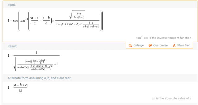
A fairly straightforward manipulation of the ‘alternate form’ output yields the expected result: ##\frac{b-a}{c}## or ##\frac{\Delta\lambda}{\lambda_c}## and gives us confidence that the formulas for ##\tan\theta_i## and ##\tan\theta_r## are valid.
Ratio Equations
From conservation of momentum along the normal, we have already established the ratio equation: $$\frac{\cos\theta_r}{\cos\theta_i}=\frac{\lambda_r}{\lambda_i}=\frac{E_i}{E_r}.$$ From the equations for ##\tan\theta_i## and ##\tan\theta_r## we can also write: $$ \frac{\tan\theta_r}{\tan\theta_i}=\frac{\lambda_i}{\lambda_r}\times\frac{\lambda_c-\lambda_r}{\lambda_c+\lambda_i}=\frac{E_r-E_o}{E_i+E_o}.$$Finally we can multiply the above pair of equations together to obtain: $$\frac{\sin\theta_r}{\sin\theta_i}=\frac{\lambda_c-\lambda_r}{\lambda_c+\lambda_i}=\frac{E_i}{E_r}\frac{E_r-E_0}{E_i+E_0}.$$
In respect of the tan ratio, it is probably worth drawing attention to the fact that the expression obtained is very similar to that determined in our previous article on elastic collisions where we determined: $$\frac{\tan\theta_r}{\tan\theta_i}=\frac{1-k}{1+k},$$where k was the ratio of stationary mass to mass in motion (pre-collision). We noted that if k was 1 (equal masses), then ##\theta_r## would be zero and thus the post-collision trajectories would be at right angles. Similarly from the tan ratio above we see that the condition for post-collision photon and electron trajectories to be at right angles is when ##E_0=E_r##. That is when the energy of the scattered photon is equal to the rest mass energy of the electron.
Worked Examples
1. Calculation of Electron Recoil Angle
Our first worked example is from the section on Compton Scattering from the website phys.libretexts.org.
An 800 keV photon collides with an electron at rest. After the collision, the photon is detected with 650 keV of energy. Find the kinetic energy and angle of the scattered electron.
From conservation of energy the kinetic energy of the electron is easily calculated as 800 – 650 = 150 keV. Electron recoil angle ##\phi## is ##90-\theta_i## which can be calculated from the reciprocal of our energy expression for ##\tan\theta_i## ie: $$\tan\phi=\tan(90-\theta_i)=\frac{E_0}{E_i+E_0}\sqrt{\frac{2E_iE_r-E_0\Delta E}{E_0\Delta E}}.$$ Taking ##E_0\approx 512\; keV##, we can simply substitute the given energies into the equation obtaining ##\tan\phi=\tan(90-\theta_i)=1.38##. Hence electron recoil angle is ##54.1^\circ##. This answer is more or less in accordance with that obtained (##54.4^\circ##) by other methods on the website whence it originates. The discrepancy may be due to rounding of intermediate answers employed en route to this solution whereas our method did not require any intermediate calculations.
2. Fixed Wavelength of Scattered Photon
(if angles for directions of motion of the electron and scattered photon are complementary)
Our second worked example is a straightforward application of the formula obtained for ##\tan\theta_r##. It can immediately be seen that this expression will be zero if the scattered photon’s wavelength is exactly equal to the electron’s Compton wavelength ##\lambda_c##. Since ##\theta_r## is defined with respect to the normal, the scattered photon will be traveling along the normal and hence at right angles to the momentum vector of the (post-collision) electron. It follows that angle of deflection and angle of electron motion (with respect to the original direction of motion of the photon) will be complementary and without further ado we have answered the homework query posted in the following thread:
https://www.physicsforums.com/threads/compton-scattering-event-proof-question.985525
3. Formula for the Electron Recoil Angle
This problem is again drawn from a PF Homework Forums question and associated thread:
https://www.physicsforums.com/threads/compton-scattering-and-conservation-of-momentum.356126
If photon scatter angle is ##\theta_d## and electron recoil angle is ##\phi##, prove that: $$\tan\phi=\frac{1}{1+\frac{hf}{m_ec^2} }\cot\left(\frac{\theta_d}{2}\right). $$
In worked example 1 we used the formula: $$\tan\phi=\tan(90-\theta_i)=\frac{E_0}{E_i+E_0}\sqrt{\frac{2E_iE_r-E_0\Delta E}{E_0\Delta E}}.$$ We just need to prove that the expression given above is equivalent to this. Since hf in the above is the incident photon’s energy ##E_i##, we can quickly establish (multiply numerator and denominator by ##m_ec^2##) that the rational part of the above expression is equivalent to ##\frac{E_0}{E_i+E_0}## and all we need do is show ##\cot\left(\frac{\theta_d}{2}\right)## is equivalent to ##\sqrt{\frac{2E_iE_r-E_0\Delta E}{E_0\Delta E}}##. The classical energy equation for Compton scattering gives: $$\cos\theta_d=1-\frac{E_0(E_i-E_r)}{E_iE_r},$$ and so all we need do is evaluate the expression: $$\cot\left(\frac{\cos^{-1}\left(1-\frac{E_0(E_i-E_r)}{E_iE_r}\right)}{2}\right).$$Wolfram Alpha duly obliges yielding the expected result – albeit requiring a little human “post processing” of the displayed result (note that we have used variables ##E_1## and ##E_2## since WA won’t take ##E_i## and ##E_r## as variables).
It’s worth noting that this particular worked example has yielded another equation for obtaining the scattering angle: $$\cot\left(\frac{\theta_d}{2}\right)=\sqrt{\frac{2E_iE_r-E_0\Delta E}{E_0\Delta E}}=\sqrt{\frac{2\lambda_c-\Delta\lambda}{\Delta\lambda}}.$$
4. Electron Recoil Angle and Energy given Angle of Deflection ##\theta_d## is twice Recoil Angle ##\phi##
This is yet another “Homework Forums” problem discussed on PF:
The information given in this problem is that a 700 keV photon (##\lambda=1.771\;pm##) scatters off an electron under the above conditions. We need to determine the electron’s recoil angle ##\phi## and its energy.
We begin by establishing some basic angle relationships which will be applicable here: $$\theta_i=90-\phi,$$ $$\theta_d=\theta_i -\theta_r⇒\theta_r=\theta_i-\theta_d=(90-\phi)-2\phi=90-3\phi.$$To determine angle ##\phi## we are going to make use of the ratio equations established above: $$\frac{\cos\theta_r}{\cos\theta_i}=\frac{\cos(90-3\phi)}{\cos(90-\phi)}=2\cos(2\phi)+1=\frac{\lambda_r}{\lambda_i},$$ $$\frac{\sin\theta_r}{\sin\theta_i}=\frac{\sin(90-3\phi)}{\sin(90-\phi)}=2\cos(2\phi)-1=\frac{\lambda_c-\lambda_r}{\lambda_c+\lambda_i}.$$From the first equation we are able to determine an expression for ##\lambda_r##:$$\lambda_r=\lambda_i(2\cos(2\phi)+1).$$Now all we need do is substitute for ##\lambda_r## in the second equation and solve for ##\cos(2\phi)##: $$2\cos(2\phi)-1=\frac{\lambda_c-\lambda_i(2\cos(2\phi)+1)}{\lambda_c+\lambda_i}$$ $$⇒\cos(2\phi)=\frac{\lambda_c}{\lambda_c+2\lambda_i}=\frac{E_i}{E_i+2E_0}\approx\frac{700}{700+2\times512}=0,406.$$Hence: $$2\phi=\theta_d=66.04^\circ⇒\phi=33.02^\circ.$$Finally to obtain the electron’s kinetic energy, we can simply determine the energy of the scattered photon and subtract it from the energy of the incident photon: $$\Delta\lambda=\lambda_c(1-\cos66.04^\circ)=1.441\;pm⇒\lambda_r=1.771+1.441=3.212\;pm.$$Hence ##E_r=386.0\; keV## and the electron’s kinetic energy will be ##700 – 386.0 = 314.0\; keV##. This result was verified by entering the energy of the incident photon and the calculated angle of deflection into the Compton scattering calculator at HyperPhysics.
5. Worked Example 4 – the “All Energy” Way.
One of the very first expressions we obtained in this article related to electron recoil angle ##\phi=90-\theta_i##: $$\tan\phi=\frac{E_0}{E_i+E_0}\sqrt{\frac{2E_iE_r-E_0\Delta E}{E_0\Delta E}}.$$ Serendipitously, in worked example 3, we had obtained an expression for ##\cot\left(\frac{\theta_d}{2}\right)## and since in this example ##\frac{\theta_d}{2}=\phi##, we may write: $$\cot\phi=\sqrt{\frac{2E_iE_r-E_0\Delta E}{E_0\Delta E}}.$$ These two equations can be divided by each other giving: $$\tan^2\theta=\frac{E_0}{E_i+E_0}⇒\tan\theta=\sqrt{\frac{E_0}{E_i+E_0}}=\sqrt{\frac{512}{700+512}}.$$Hence we obtain ##\phi=33.02^\circ## and ##\theta_d=66.04^\circ## as before. Energy of the recoiling electron follows as in worked example 4 above.
6. Worked Example 6
“Gamma rays (high energy photons) of energy 1.02 MeV are scattered from electrons that are initially at rest. If the scattering is symmetric, that is ##\theta_d=\phi## find the scattering angle and the energy of the scattered photon.”
The diagram for this problem follows. Note that we have introduced a set of axes parallel and perpendicular (normal) to the vector representing the post-collision motion of the electron. The incident and refracted angles ##\theta_i## and ##\theta_r## are measured with respect to the normal (y-axis). Their relation to the direction of motion of the electron ##\phi## and scattering angle ##\theta_d=\phi## is shown on the diagram and derives from simple geometry.
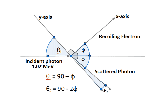
We begin by applying one of the ratio equations derived in this article: $$\frac{\cos\theta_r}{\cos\theta_i}=\frac{E_i}{E_r}⇒\frac{\cos(90-2\phi)}{\cos(90-\phi)}=\frac{E_i}{E_r}⇒2\cos\phi=\frac{E_i}{E_r}⇒E_r=\frac{E_i}{2\cos\phi}.$$From the standard scattering equation we have: $$1-\cos\theta_d=1-\cos\phi=E_0\left(\frac{1}{E_r}-\frac{1}{E_i}\right)=E_0\left(\frac{2\cos\phi}{E_i}-\frac{1}{E_i}\right)=\frac{E_0}{E_i}(2\cos\phi-1).$$ Hence we obtain: $$\cos\phi=\frac{E_i+E_0}{E_i+2E_0}.$$ Finally plugging in the numbers ##E_0=512\;keV## and ##E_i=1020\;keV## we obtain ##\phi=41.45^\circ## and ##E_r=\frac{E_i}{2\cos\phi}=680.44\;keV.##
Summary and Conclusions
In this article we have revisited the standard theory relating to Compton scattering and in addition have explored additional parameters by examining the photon/electron interaction from the vantage of a set of axes defined parallel and perpendicular to the direction of motion of the electron. Emerging from this analysis we obtained the following formulae for the photon’s ‘incident’ and ‘refracted’ angles respectively: $$\tan\theta_i=\frac{\lambda_c+\lambda_i}{\lambda_i}\sqrt{\frac{\Delta\lambda}{2\lambda_c-\Delta\lambda}}=\frac{E_i+E_0}{E_0}\sqrt{\frac{E_0\Delta E}{2E_iE_r-E_0\Delta E}},$$ $$\tan\theta_r=\frac{\lambda_c-\lambda_r}{\lambda_r}\sqrt{\frac{\Delta\lambda}{2\lambda_c-\Delta\lambda}}=\frac{E_r-E_0}{E_0}\sqrt{\frac{E_0\Delta E}{2E_iE_r-E_0\Delta E}}.$$ We have tested these formulas first by using them to verify the standard Compton relationship on scattering angle and then by way of some worked examples whereby we reach the same answers as are obtained using conventional methods.
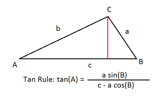
Appendix: The Tan Rule
Most readers will be familiar with the sine rule and cosine rule. The ‘tan rule’ appears to be something of an omission in terms of the fact that it is not commonly taught in school curricula for some reason. So in the diagram below where the givens are sides a and c along with angle B, there would normally be a two-step process to find angle A. First, determine side b using the cosine rule and once that is known, calculate angle A using the sine rule. The illustration below indicates this is not necessary as a single rule will suffice to determine angle A from the 3 givens.
Acknowledgments
I would like to sincerely thank a number of PF users who took the time to go through the draft article and make suggestions for its improvement. As a result, the original version has undergone a comprehensive revision mainly directed towards presenting the various equations in their energy equivalent forms following the unanimous consensus of the reviewers. As can be seen, I have (with the kind permission of the contributors) included most of the review comments within the context of the article and at this point express my sincere gratitude to PF users edguy99, vanhees71, vela, jtbell and Dr_Nate. This has been a collaborative effort and should perhaps even be presented as a multi-author article if that is possible.
Without the assistance of the Wolfram Alpha computational engine, some of the algebraic manipulations required in the article would probably not have been possible. Or at the very least would have taken years to complete.
References
| [1] | Arthur H Compton. compton.pdf. https://history.aip.org/history/exhibits/gap/PDF/compton.pdf, May 1923. (Accessed on 04/11/2020). [ bib ] |
| [2] | Wikipedia contributors. Compton wavelength – Wikipedia. https://en.wikipedia.org/wiki/Compton_wavelength. (Accessed on 04/11/2020). [ bib ] |
| [3] | Wolfram Alpha. Solving for the angle of refraction. (Accessed on 04/07/2020). [ bib ] |
| [4] | Wolfram Alpha. Verifying the equations for the incident and refracted angles. (Accessed on 04/07/2020). [ bib ] |
| [5] | Paul D’Alessandris. Source for Worked Example 1. (Accessed on 04/11/2020). [ bib ] |
| [ 6] | PF User jisbon & Homework Helpers. Compton scattering event (proof question) | physics forums.https://www.physicsforums.com/threads/compton-scattering-event-proof-question.985525/. (Accessed on 04/11/2020). [ bib ] |
| [7] | PF user Nusc & PF Homework Helpers. Compton scattering and conservation of momentum | physics forums.https://www.physicsforums.com/threads/compton-scattering-and-conservation-of-momentum.356126/. (Accessed on 04/11/2020). [ bib ] |
| [8] | PF user akennedy & Homework Helpers. Compton effect problem – find angle and energy of a scattered electron | physics forums.https://www.physicsforums.com/threads/compton-effect-problem-find-angle-and-energy-of-scattered-electron.745785/ (Accessed on 04/11/2020).[ bib ] |
| [9] | Hyperphysics. Relativistic energy. http://hyperphysics.phy-astr.gsu.edu/hbase/Relativ/releng.html. (Accessed on 04/28/2020). [ bib ] |
| [10] | HyperPhysics. Compton scattering calculator.http://hyperphysics.phy-astr.gsu.edu/hbase/quantum/compton.html#c1. (Accessed on 04/28/2020). [ bib ] |
- BSc (Elec Eng) University of Cape Town, HDE University of South Africa
- Maths and Science Tutor, Florida Park, Johannesburg
- Research areas (personal interest): Hydrogen / Hydrogen-like spectra. Historical Maths.
- Wikipdedia contributions: Ptolemy’s Theorem, Diophantus II.VIII, Continuous Repayment Mortgage


Leave a Reply
Want to join the discussion?Feel free to contribute!