Weak Values Part 2: The Quantum Cheshire Cat Experiment

In a previous Insight, Weak Values Part 1: “Asking Photons Where They Have Been,” I showed different methods for computing the relative intensities in the weak measurements done by Danan, Farfurnik, Bar-Ad, and Vaidman (DFBV)[1]. In that experiment, DFBV had a weak transverse signal, created by mirrors oscillating with small amplitudes transverse to the beam path through an interferometer, piggyback on a strong longitudinal signal[2], i.e., the beam path through the interferometer. The relative intensities of that weak signal were obtained from the first-order contributions to the wave function in all three computational approaches. In the case of the Two-State Vector Formulation (TSVF) of quantum mechanics (QM), the weak values were then used to infer an answer to the question, “Where were the photons between emission at the Source and detection at the detector?” In this Insight I will analyze another weak measurement done by Denkmayr et al.[3] called the quantum Cheshire Cat experiment. In this experiment we will see how the implications of weak values can be destroyed when they are obtained using second-order contributions to the interaction.

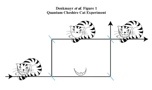
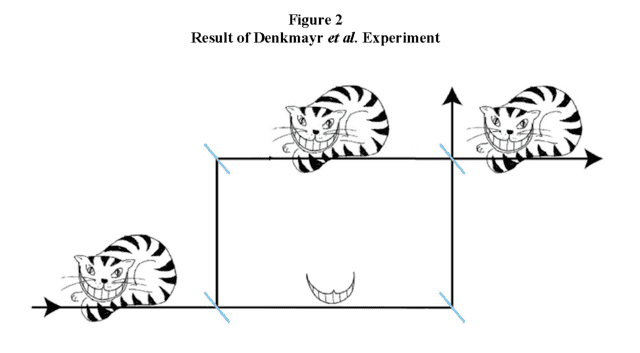
Using a neutron interferometer, Denkmayr et al. attempted to instantiate the quantum Cheshire Cat experiment. In a quantum Cheshire Cat experiment[4], a particle can be spatially separated form one of its properties just as the Cheshire Cat can be spatially separated from its grin in the Lewis Carroll story Alice’s Adventures in Wonderland[5] (see their Figure 1 below). If an experiment were to be performed like this, Corrêa et al. showed that it could be explained by quantum interference[6], but as we will see Denkmayr et al. failed to instantiate the quantum Cheshire Cat (qCC) experiment even though they measured the correct weak values. Instead of Figure 1, what they obtained was their modified Figure 2 (below) because of an unavoidable second-order contribution from the weak magnetic field. I will start by deriving the QM intensities for their experiment, then I will explain how the second-order contribution destroys the qCC implication of the weak values[7].

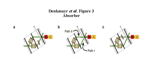
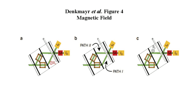
The experiment is summarized in Denkmayr et al.’s Figures 3 and 4 below. To understand the essential elements of the experiment, you need to know that spin rotators create [itex] \mid S_x + \rangle [/itex] (or  [itex] \mid + \rangle [/itex] for short) on path I and  [itex] \mid S_x – \rangle [/itex] (or [itex] \mid – \rangle [/itex] for short) on path II (brown boxes in Figure 3) just after the neutrons pass through the first beam splitter (entering from the left in Figure 3). Path I is the “lower path” and path II is the “upper path.” The two detectors are O (labeled by I_o in yellow boxes of Figures 3 & 4) and H (labeled by I_H in yellow box of Figure 4). A [itex] \mid – \rangle [/itex] spin selector immediately precedes the detector O (red box labeled SA) while the entire signal is sampled at H. The grey bar in Figures 3 & 4 just before the second beam splitter is used to adjust the relative phase [itex]\chi [/itex] between the two paths so that the signal is equally divided coming out of the second beam splitter with [itex]\chi = 0[/itex]. This is the configuration used to measure the weak values which are necessary (but not sufficient as it turns out) to establish the qCC, as we will see. Thus, when a partial (weak) absorber (brown bar in Figure 3) is placed in path I it diminishes the [itex] \mid + \rangle [/itex] amplitude contributing to the amplitude going to the spin selector. But, the [itex] \mid – \rangle [/itex] spin selector deletes that effect on the amplitude going to O, so there is no change in the intensity at O. However, when the partial absorber is placed in path II it diminishes the [itex] \mid – \rangle [/itex] amplitude contributing to the amplitude going to the spin selector, so this decrease in the amplitude reaches O giving rise to a slight decrease in the intensity at O. The corresponding weak values are for projection operators in each path, i.e., [itex] \langle \Pi _I \rangle _W = 0 [/itex] and [itex] \langle \Pi _{II} \rangle _W = 1 [/itex]. The experimenters therefore conclude that the neutrons reaching O are taking path II, i.e., “a minimally disturbing measurement will find the Cat in the upper beam path … .” This part of the experiment is straightforward and requires no detailed analysis. It is the second part of the experiment, i.e., the introduction of a weak magnetic field B_z, that yields the controversial part of the conclusion, i.e., “… while its grin will be found in the lower one.”

To establish the location of the z component of the neutrons’ spin reaching detector O, a weak magnetic field B_z is introduced to each path in turn. The weak values [itex] \langle \sigma _z \Pi _I \rangle _W = 1 [/itex] and [itex] \langle \sigma _z \Pi _{II} \rangle _W = 0 [/itex] should imply that the z component of the neutrons’ spin reaching O took path I through the interferometer if they are measured properly, i.e., using a weak enough B_z where “weak enough” will turn out to mean “linear interaction,” as we will see. Let’s derive the theoretical amplitudes and intensities at detector O and then have a look at the data.

We will compute the amplitude for each path through the interferometer using neutron optics. There are two differences between neutron optics and photon optics for our interferometer, i.e., the neutron amplitude does not acquire a factor of i after reflections and the neutron spin state is affected by B_z. Let’s start by finding the amplitude coming from the second beam splitter towards detectors H and O with B_z = 0 and no spin selector (no red box labeled SA in Figure 4b).

In the upper path (II), after the first beam splitter and spin rotator our amplitude is [itex] \frac{1}{\sqrt{2}} \mid – \rangle [/itex], since a 50-50 beam splitter introduces a factor of [itex] \frac{1}{\sqrt{2}} [/itex] and the spin rotator creates [itex] \mid – \rangle [/itex].  Likewise in the lower path (I), after the first beam splitter and spin rotator our amplitude is [itex] \frac{1}{\sqrt{2}} \mid + \rangle [/itex]. These each acquire another factor of [itex] \frac{1}{\sqrt{2}} [/itex] passing through the second beam splitter so the amplitude at H or O is

\begin{equation} A_{bare} = \frac{1}{2} \left( \mid + \rangle + \mid – \rangle \right) \label{noB} \end{equation}

[itex] \mid A_{bare} \mid ^2 = \frac{1}{2} [/itex] tells us that the signal is split evenly between H and O. Further, [itex]\mid \langle \pm \mid A_{bare} \rangle \mid ^2 = \frac{1}{4} [/itex] tells us that the signal is also split evenly between [itex] \mid – \rangle [/itex] and  [itex] \mid + \rangle [/itex] at each of H and O. Thus, [itex] I^{REF} = \frac{1}{4} [/itex] for the intensity at O. Now let’s add a magnetic field B_z to the upper path (II) after the spin rotator.

The magnetic field effect is given by the unitary operator [itex] e^{i \sigma _z \alpha /2} [/itex] on the amplitude at that point, as shown in their Eq (8). [itex]\sigma _z [/itex] is the Pauli spin z matrix and [itex]\alpha [/itex] is proportional to the magnetic field strength. Accordingly, the magnetic field effect is

\begin{equation} e^{i \sigma _z \alpha /2} \mid – \rangle = \left( I cos\left(\frac{\alpha}{2}\right) + i\sigma _z sin\left(\frac{\alpha}{2}\right)\right)\mid – \rangle = cos\left(\frac{\alpha}{2}\right) \mid – \rangle \: – \: i sin\left(\frac{\alpha}{2}\right)\mid + \rangle \label{Op1} \end{equation}

since [itex] \sigma _z \mid – \rangle \: = \: -\mid + \rangle [/itex]. Likewise, [itex] \sigma _z \mid + \rangle \: = \: -\mid – \rangle [/itex]. That is,

\begin{equation} \sigma _z = \begin{pmatrix} 1 & 0\\0 & -1 \end{pmatrix}   \label{spinz} \end{equation}

while

\begin{equation} \sigma _x = \begin{pmatrix} 0 & 1\\1 & 0 \end{pmatrix}   \label{spinx} \end{equation}

in the eigenbasis of [itex] \sigma _z [/itex]. The orthonormal eigenstates of [itex] \sigma _x [/itex] are

\begin{equation} \mid + \rangle = \frac{1}{\sqrt{2}} \begin{pmatrix} 1\\1 \end{pmatrix}   \label{x+} \end{equation}

and

 \begin{equation} \mid – \rangle = \frac{1}{\sqrt{2}} \begin{pmatrix} -1\\1 \end{pmatrix}   \label{x} \end{equation}

with eigenvalues +1 and -1, respectively, which you can check by explicit matrix multiplication, e.g.,

\begin{equation} \sigma _x \mid – \rangle = \begin{pmatrix} 0 & 1\\1 & 0 \end{pmatrix} \frac{1}{\sqrt{2}} \begin{pmatrix} -1\\1 \end{pmatrix} = \frac{1}{\sqrt{2}}  \begin{pmatrix} 1\\-1 \end{pmatrix}  = \: – \mid – \rangle \label{eigenx} \end{equation}

Thus,

\begin{equation} \sigma _z \mid – \rangle = \begin{pmatrix} 1 & 0\\0 & -1 \end{pmatrix} \frac{1}{\sqrt{2}} \begin{pmatrix} -1\\1 \end{pmatrix} = \frac{1}{\sqrt{2}}  \begin{pmatrix} -1\\-1 \end{pmatrix}  = \: – \mid + \rangle \label{sigmazx} \end{equation}

and

\begin{equation} \sigma _z \mid + \rangle = \begin{pmatrix} 1 & 0\\0 & -1 \end{pmatrix} \frac{1}{\sqrt{2}} \begin{pmatrix} 1\\1 \end{pmatrix} = \frac{1}{\sqrt{2}}  \begin{pmatrix} 1\\-1 \end{pmatrix}  = \:-  \mid – \rangle \label{sigmazx+} \end{equation}

Therefore, the amplitude at H or O without the spin selector SA and B_z in the upper path (II) is

\begin{equation} A^{MAG} _{II} = \frac{\mid + \rangle}{2} + \frac{1}{2}\left( cos\left(\frac{\alpha}{2}\right) \mid – \rangle \: – \: i sin\left(\frac{\alpha}{2}\right)\mid + \rangle \right) \label{AIInoSA} \end{equation}

We still have the overall signal divided evenly between H and O since

\begin{equation} I^{MAG} _{II} = \mid A^{MAG} _{II} \mid ^2 = \frac{1}{4} + \frac{1}{4}sin^2\left(\frac{\alpha}{2}\right) + \frac{1}{4}cos^2\left(\frac{\alpha}{2}\right) = \frac{1}{2} \label{IuppernoSA} \end{equation}

However, the intensity due to [itex]\mid + \rangle [/itex] is

\begin{equation} I^{MAG} _{II/+} = \frac{1}{4} + \frac{1}{4}sin^2\left(\frac{\alpha}{2}\right)  = \frac{1}{4} \left( 2 – cos^2\left(\frac{\alpha}{2}\right) \right) \label{+amount} \end{equation}

while the intensity due to [itex]\mid – \rangle [/itex] is

\begin{equation} I^{MAG} _{II/-} = \frac{1}{4}cos^2\left(\frac{\alpha}{2}\right) \label{-amount} \end{equation}

For [itex]\alpha = 0[/itex] the signal is evenly divided and as [itex] \alpha \rightarrow \pi [/itex] we have [itex] I^{MAG} _{II/+} \rightarrow \frac{1}{2} [/itex] and [itex] I^{MAG} _{II/-} \rightarrow 0 [/itex]. That is B_z converts all of the [itex]\mid – \rangle [/itex] amplitude in path II to [itex]\mid + \rangle [/itex].

Likewise, placing B_z in the lower path (I) results in

\begin{equation} A^{MAG} _{I} = \frac{\mid – \rangle}{2} + \frac{1}{2}\left( cos\left(\frac{\alpha}{2}\right) \mid + \rangle \: – \: i sin\left(\frac{\alpha}{2}\right)\mid – \rangle \right) \label{AInoSA} \end{equation}

for the amplitude at H or O, which is just Eq(\ref{AIInoSA}) with [itex] \mid + \rangle [/itex] and [itex] \mid – \rangle [/itex] switched. Thus, as  [itex] \alpha \rightarrow \pi [/itex] we have [itex] I^{MAG} _{I/-} \rightarrow \frac{1}{2} [/itex] and [itex] I^{MAG} _{I/+} \rightarrow 0 [/itex]. That is B_z converts all of the [itex]\mid + \rangle [/itex] amplitude in path I to [itex]\mid – \rangle [/itex].

It is now easy to add the spin selector between the second beam splitter and O, since that just selects the [itex] \mid – \rangle [/itex] part of the amplitude at that point. Mathematically, the spin selector effect on the amplitude at that point is given by [itex] \mid – \rangle \langle – \mid [/itex], so the amplitude at O when B_z is placed in the upper path (II) is given by

\begin{equation} A^{MAG} _{II/O} = \frac{1}{2}cos\left(\frac{\alpha}{2}\right) \mid – \rangle \label{IItotalO} \end{equation}

and the intensity (neutrons per second) at O is then

\begin{equation} I^{MAG} _{II/O} = \mid A_{II/O} \mid ^2 = \frac{1}{4}cos ^2\left(\frac{\alpha}{2}\right) = I^{REF}cos ^2\left(\frac{\alpha}{2}\right)  \label{IIO} \end{equation}

their Eq(14). When we place B_z in the lower path (I)

\begin{equation} A^{MAG} _{I/O} = \frac{\mid – \rangle}{2} – \frac{i}{2} sin\left(\frac{\alpha}{2}\right)\mid – \rangle \label{ItotalO} \end{equation}

so the intensity at O is then

\begin{equation} I^{MAG} _{I/O} = \frac{1}{4} \left( 2 – cos^2\left(\frac{\alpha}{2}\right) \right) = \frac{1}{8}\left(3 – cos \left(\alpha \right)\right) = \frac{I^{REF}}{2}\left(3 – cos \left(\alpha \right)\right)  \label{IO} \end{equation}

their Eq(13) with [itex] \chi = 0 [/itex]. Now let’s look at the data.

The authors give I^REF = 11.25(5) counts per second (cps) at O. Again, I^REF  is the intensity (neutrons per second) at O when B_z is zero and [itex]\chi = 0 [/itex]. Their magnetic field strength parameter [itex]\alpha = 20^o [/itex], so plugging this into Eq(\ref{IIO}) we obtain a theoretical prediction of 10.91(5) cps, which agrees with their measured value of 10.93(6) cps. Thus, when weak B_z is introduced in the upper path (II) (corresponding to small [itex]\alpha [/itex]), we see a small decrease in the intensity at O (where, again, only [itex]\mid – \rangle [/itex] is sampled) due to some of the  [itex]\mid – \rangle [/itex] amplitude in the upper path being converted to  [itex]\mid + \rangle [/itex] amplitude by the magnetic field there. The decrease is given by

\begin{equation} I^{MAG} _{II/O} \approx I^{REF} \left(1 – \left(\frac{\alpha}{2}\right)^2 \right) \label{IIOweak} \end{equation}

or about a 3% reduction in I^REF, i.e., 11.25 – 0.34 = 10.91.

Plugging I^REF and [itex]\alpha [/itex] into Eq(\ref{IO}) we obtain a theoretical prediction of 11.59(5) cps in agreement with their measured value of 11.57(6) cps. Thus, when weak B_z is introduced in the lower path (I) (corresponding to small [itex]\alpha [/itex]), we see a small increase in the intensity at O (where, again, only [itex]\mid – \rangle [/itex] is sampled) due to some of the  [itex]\mid + \rangle [/itex] amplitude in the lower path being converted to  [itex]\mid – \rangle [/itex] amplitude by the magnetic field there. The increase is given by

\begin{equation} I^{MAG} _{I/O} \approx I^{REF} \left(1 + \left(\frac{\alpha}{2}\right)^2 \right) \label{IOweak} \end{equation}

or about a 3% increase in I^REF, i.e., 11.25 + 0.34 = 11.59. Thus, we have very nice agreement between QM theory and experiment. However, the results don’t suggest anything like qCC (separation of a particle and one of its properties), since we have exactly a 3% effect on the intensity at O whether B_z is in path I or II, which means we have Figure 2 instead of Figure 1. Let’s look at the corresponding evaluation using weak values and see where that goes awry.

The authors write [itex] I^{MAG} _j [/itex] at O in terms of weak values as (their Eq(10))

\begin{equation} I^{MAG} _j = \mid \langle \Psi _f  \mid \Psi _i \rangle \mid ^2 \left[1 – \frac{\alpha^2}{4}\langle \Pi _j \rangle _W + \frac{\alpha^2}{4} \mid \langle \sigma _z \Pi _j \rangle _W \mid ^2 \right] \label{10} \end{equation}

where [itex] \mid \langle \Psi _f  \mid \Psi _i \rangle \mid ^2 = I^{REF} [/itex], [itex] \langle \Pi _I \rangle _W = 0 [/itex], [itex] \langle \Pi _{II} \rangle _W = 1 [/itex], [itex] \langle \sigma _z \Pi _I \rangle _W = 1 [/itex], and [itex] \langle \sigma _z \Pi _{II} \rangle _W = 0 [/itex]. Notice that the weak values turn Eq(\ref{10}) into Eqs(\ref{IIOweak} & \ref{IOweak}), so indeed we have established a weak enough B_z to render the weak values relevant. However, the problem for the qCC interpretation of our weak values is obvious — we need [itex] \langle \Pi _{II} \rangle _W = 1 [/itex] to establish the effect of B_z in path II where there should be no effect. Where did this contribution originate?

Consider the effect of [itex] e^{i \sigma _z \alpha /2} [/itex] on the amplitude in path j to lowest (linear) order in [itex]\alpha [/itex], i.e.,

\begin{equation} e^{i \sigma _z \alpha /2} \approx I + i\sigma _z \alpha /2 \label{operator} \end{equation}

Accordingly, when weak B_z is placed in path j all that matters to lowest order in [itex]\alpha [/itex] for understanding the effect on the amplitude is [itex] i\sigma _z \alpha /2 [/itex], which is characterized by [itex] \langle \sigma _z \Pi _{j} \rangle _W [/itex]. Notice that by “weak” we mean “weak enough” to exclude measureable/observable second-order (quadratic) effects in [itex]\alpha [/itex]. So, with weak B_z in path I, given the effect of [itex]\sigma _z [/itex] on [itex]\mid + \rangle [/itex] and the [itex]\mid – \rangle [/itex] spin selector immediately preceding O, there is a discernible effect of the interaction Hamiltonian on the amplitude and [itex] \langle \sigma _z \Pi _I \rangle _W = 1 [/itex] captures this fact nicely. In contrast, with weak B_z in path II, the effect of the interaction Hamiltonian on the amplitude is given by I, i.e., [itex] e^{i \sigma _z \alpha /2} [/itex] has no effect on the amplitude at O when B_z is in path II, and [itex] \langle \sigma _z \Pi _{II} \rangle _W = 0 [/itex] captures this fact nicely.

But, this is not what we observed. As we showed above, there is a reduction in the intensity at O for weak B_z in path II no matter how weak we make B_z. The reason for this is that the intensity is obtained from the amplitude squared, not the amplitude. So, when we want to ask a question about the empirical effect of the interaction Hamiltonian on the amplitude for weak B_z in path II, we must keep the quadratic term in [itex]\alpha [/itex] coming from [itex] e^{i \sigma _z \alpha /2} [/itex], because ultimately that term will be as important observationally, i.e., for the intensity, as the linear term in [itex]\alpha [/itex] coming from [itex] e^{i \sigma _z \alpha /2} [/itex] no matter how weak we make B_z. That is,

\begin{equation} e^{i \sigma _z \alpha /2} \approx I + i\sigma _z \alpha /2 – I \alpha ^2 /8 = I \left(1 – \alpha ^2 /8 \right) + i\sigma _z \alpha /2 \label{operator2} \end{equation}

is the form that gives us Eq(\ref{10}). So, the term [itex]\frac{\alpha^2}{4} \mid \langle \Pi _j \rangle _W \mid ^2 [/itex] in [itex] I^{MAG} _j [/itex] that destroys the qCC interpretation comes from the quadratic contribution to the expansion of [itex] e^{i \sigma _z \alpha /2} [/itex]. And, this quadratic contribution is equal to the linear contribution when computing the intensity. Thus, while Denkmayr et al. failed to instantiate qCC, their experiment does reveal an interesting fact, i.e., weak values can be measured via quadratic interaction, but weak values measured in this fashion may not have straightforward ontological implications per TSVF.

Update: One of the authors of Denkmayr et al. (A. Matzkin) is coauthor on a recent publication [11] that concludes, “The QCC effect as predicted theoretically has not yet been experimentally observed, as the experimental realizations done so far have not been able to properly implement the weak measurement protocol.” Thus, an author of Denkmayr et al. admits they did not experimentally observe the QCC effect.

To recap my Insights thus far, in order to understand the problem that quadratic interaction in a weak measurement creates in making ontological inferences with weak values, I first analyzed a weak measurement that used linear interaction strength. Before introducing weak values at all, I had to introduce TSVF’s use of retrocausality. To explain retrocausality, I first derived the blockworld implication of the relativity of simultaneity from special relativity. And, to motivate the relativity of simultaneity, I started my Insights by explaining length contraction and time dilation per special relativity.

In my next Insight, I will explain the quantum liar experiment[8] as an instantiation of the Mermin device[9]. To do that I will first explain the quantum state used in the Mermin device per Dehlinger & Mitchell’s “Entangled photons, nonlocality, and Bell inequalities in the undergraduate laboratory”[10].

1. Danan, A., Farfurnik, D., Bar-Ad, S., & Vaidman, L.: Asking Photons Where They Have Been. Physical Review Letters 111, 240402 (2013) http://arxiv.org/abs/1304.7469.
2. The electromagnetic wave for this “longitudinal signal” is still a transverse wave in the electric and magnetic fields, of course.
3. Denkmayr, T., Geppert, H., Sponar, S., Lemmel, H., Matzkin, A., Tollaksen, J., & Hasegawa, Y.: Observation of a quantum Cheshire Cat in a matter-wave interferometer experiment. Nature Communications, DOI: 10.1038/ncomms5492 (29 Jul 2014).
4. Tollaksen, J.: Quantum Reality and Nonlocal Aspects of Time. PhD thesis, Boston University. (2001); Matzkin, A. & Pan, A. K.: Three-box paradox and ‘Cheshire cat grin’: the case ofspin-1 atoms. Journal of Physics A: Mathematical and Theoretical 46, 315307 (2013); Aharonov, Y., Popescu, S., Rohrlich, D. & Skrzypczyk, P.: Quantum CheshireCats. New Journal of Physics 15, 113015 (2013).
5. Carroll, L.: Alice’s Adventures in Wonderland. MacMillan Press, United Kingdom (1865).
6. Corrêa, R., Santos, M.F., Monken, C.H., & Saldanha, P.L.: ‘Quantum Cheshire Cat’ as Simple Quantum Interference. New Journal of Physics 17, 053042 (2015) http://arxiv.org/abs/1409.0808.
7. Stuckey, W.M., Silberstein, M., & McDevitt, T.: Concerning Quadratic Interaction in the Quantum Cheshire Cat Experiment. International Journal of Quantum Foundations 2, 17-31 (2016)http://www.ijqf.org/wps/wp-content/uploads/2015/12/IJQF2016v2n1p2.pdf.
8. Elitzur, A., & Dolev, S.: Quantum Phenomena within a New Theory of Time: In: Elitzur, A., Dolev, S., & Kolenda, N. (eds.) Quo Vadis Quantum Mechanics? p 325, Springer, New York (2005).
9. Mermin, N.D.: Bringing home the atomic world: Quantum mysteries for anybody. American Journal of Physics 49, 940-943 (1981).
10. Dehlinger, D., & Mitchell, M.W.: Entangled photons, nonlocality, and Bell inequalities in the undergraduate laboratory. American Journal of Physics 70, 903-910 (2002).
11. Q. Duprey, Q., Kanjilal, S., Sinha, U., Home, D., & Matzkin, A.: The Quantum Cheshire Cat effect: Theoretical basis and observational implications. Annals of Physics 391, 1–15 (2018).