How Bayesian Inference Works in the Context of Science

Confessions of a moderate Bayesian part 3

Read part 1: How to Get Started with Bayesian Statistics
Read part 2: Frequentist Probability vs Bayesian Probability

Bayesian statistics by and for non-statisticians

https://www.cafepress.com/physicsforums.13280237

Background

One of the things that I like about Bayesian statistics is that it rather closely matches the way that I think about science, although of course in a more formal manner. Also, many of the more important concepts of scientific philosophy arise naturally and are enforced naturally when using Bayesian methods. I have a decidedly anti-philosophy philosophy of science, so I like being able to reduce scientific philosophy to features of a mathematical framework. Particularly when the mathematical framework does a better job than the philosophers themselves.

I will use an example of a data set of 40000 flips of a real coin (a US dime) under two different conditions, one person that always started the coin heads up and the other that always started the coin tails up. This data is taken from:

https://www.stat.berkeley.edu/~aldous/Real-World/coin_tosses.html

To set up the data and the libraries we use I will run this in R

library(rstanarm)
library(ggplot2)
library(bayesplot)
library(emmeans)
library(bayestestR)
inv_logit <- function(x) { return(exp(x)/(1+exp(x))) }
logit <- function(x) { return(log(x/(1-x))) }

dat <- read.csv("coin_tosses.csv")
summary(dat)

From this we see that there were 20217 flips that landed Heads and 19783 landed Tails with 40000 total flips, 20000 starting from Heads and 20000 starting from Tails.

We are interested in hypotheses about the probability of the coin flip landing Tails. For convenience, let’s define ##X=P(Tails)##. So ##X=0.5## is a perfectly fair coin, ##X=1.0## is a coin that always lands Tails, and ##X=0.0## is a coin that always lands Heads. We might also specify that a coin that is in the range ##X \in [0.49,0.51]## is practically equivalent to a fair coin.

Bayesian science

Bayesian inference is centered around Bayes’ theorem: $$P(H|E) = \frac{P(E|H) \ P(H)} {P(E)}$$ where ##H## is your scientific hypothesis and ##E## is the evidence. So ##P(H|E)## is the probability of the hypothesis given the evidence, which is called the posterior probability. ##P(H)## is the probability of the hypothesis before considering the new evidence which is called the prior probability. The factor ##P(E|H)/P(E)## is the strength of the evidence and describes how much the evidence changes our uncertainty.

Posterior probability

In science, usually we want to “prove” our hypothesis, so we try to gather evidence that shows that our hypothesis is valid. In Bayesian inference this means that we want to show that ##P(H|E)## is large (close to 1). To me, this is very straightforward. I have a hypothesis, but I am not very certain about it. So I gather data and hopefully become more certain about my hypothesis. To me, assigning a probability to a hypothesis makes sense and matches how I think of the scientific method.

In contrast, since we have no infinite pool of universes to test and determine if the hypothesis is true or false in each universe, there is simply no sensible way to assign a long-run frequency to the hypothesis itself. So it cannot be treated as a legitimate frequentist probability. Instead, we make a “null hypothesis”, ##H_0##, which is a hypothesis that we usually don’t believe but we use as a kind of scientific “strawman” default hypothesis. Then we calculate ##P(E|H_0)## which is the famous p-value. This p-value, ##P(E|H_0)##, clearly has nothing to do with the actual hypothesis of interest, ##H##, but ##p<0.05## is often (mis-)interpreted as demonstrating the validity of ##H## anyway.

Posterior probability for coin flip example

Overall the data has 19783 Tails, so we would not agree with a hypothesis that ##X \approx 0.6## but we would be willing to accept a hypothesis that ##X \approx 0.495##. In fact, for any ##X## we can estimate ##P(X|E)## and thus get our posterior distribution.

post <- stan_glm(End ~ 1, data = dat, family = binomial(link = "logit"))

mcmc_dens(post, transformations = inv_logit) +
labs(title = "Posterior distribution for X=P(Tails)", x = "P(X|E)", y = "Probability density")

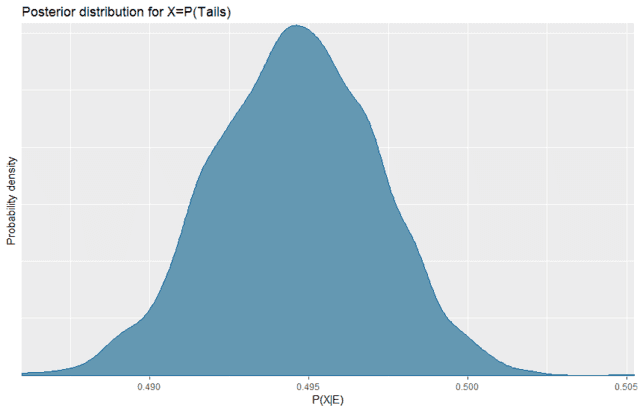
From this it looks like with 40000 flips we have a fairly precise estimate of the probability of getting Tails, which is in the range 0.49 to 0.50. To be more exact, we can calculate the Highest Posterior Density (HPD) interval which is the smallest interval such that ##P(X\in [HPD] | E)=0.95##.

summary(emmeans(post, specs = ~ 1, type = "response"))

Gives us

1        prob lower.HPD upper.HPD
overall 0.495      0.49     0.499

Results are back-transformed from the logit scale
HPD interval probability: 0.95

So the HPD is [0.490,0.499] and notably 0.5 is outside of the HPD. To misuse frequentist terminology, this would imply that the coin is significantly unfair.

But with a Bayesian posterior we can do more than just calculate the HPD. For example, with the practical equivalence criteria described above, we can calculate ##P(X \in [0.49,0.51]|E) = 0.969##. Meaning that even though the coin is probably not exactly fair it is also probably close enough to fair to be considered equivalent for all practical purposes. The calculation is as follows:

post.df <- as.data.frame(post)
post.df$ptails <- inv_logit(post.df$`(Intercept)`)
ecdf(post.df$ptails)(0.51)-ecdf(post.df$ptails)(0.49)

Prior probability

So the end result of a Bayesian analysis, ##P(H|E)##, is scientifically natural (to me at least), but what about the stuff on the right hand side of Bayes’ theorem. Does that also fit in scientifically? The thing that causes the most consternation in Bayesian inference is the prior probability. In my opinion, it is simultaneously the best and the worst part of the Bayesian approach.

The good

The prior probability, ##P(H)##, represents our uncertainty about the hypothesis without looking at the new evidence, ##E##, but it can be informed by other evidence from previous studies, expert opinion, theoretical arguments, etc.

Ideally, each scientific study should begin by investigating the previous literature on the topic or related topics. Other information can be included as well, such as the informed opinion of recognized experts. The synthesis of this data is the prior which is a summary of the current state of knowledge on the topic before considering the new data.

A few years back when CERN produced experimental evidence that neutrinos went faster than c, there were a lot of people who were very skeptical of the result. Were the skeptics scientifically justified in their assumption?

According to Bayes they were scientifically justified. There was a wealth of previous data on the topic, and this wealth of previous data led to a strong prior against FTL neutrinos. Although the evidence contradicted this prior it was not so strong that it completely reversed the strong prior. Instead, it merely weakened the strong prior to weaker prior still firmly against FTL neutrinos. These researchers knew the previous evidence and considered the new evidence in context.

It is typically possible to start with a non-informative prior. That is a prior that represents complete ignorance on the topic and essentially allows the data to speak for itself. In my opinion, this is a practice to avoid as much as possible. The act of forming a good prior requires a thorough investigation of the existing literature and a careful consideration of the model to be studied, while a non-informative prior ignores all of that. Also, for technical reasons often non-informative priors have poor convergence.

However, there is one thing that does argue for the use of non-informative priors, and that is the fact that many frequentist tests are equivalent to Bayesian tests with non-informative priors. Nevertheless, I think it is usually best to use informative priors which should be carefully justified through an extensive review of the literature.

The bad

Unfortunately, some Bayesian methods are very sensitive to the choice of prior. This can be problematic if either dramatically different conclusions are reached with minor differences in the priors, or if the priors overwhelm even large amounts of data.

One approach is to use multiple priors. One prior can be minimally informative, another could represent the best estimate from the literature, and another one or more could represent strong opinions held by different opinion leaders.

The ugly

One of the biggest problems with priors is simply that they can be difficult for researchers to adequately specify. Often the priors on a model require the specification of one or more quantities that are not well known. These can be quantities that are necessary for operation of the statistics, but not predicted or described by the relevant theory or even are unmeasurable. They can also be quantities that are not of interest to the community and so are simply not discussed in the published literature.

Improving this aspect is largely a matter of training and familiarity with developing good priors. It can also be improved by the development of specific statistical methods with more intuitive priors. Often a model can be transformed to a different representation and the prior in the transformed representation may be easier for users to specify.

Prior probability for coin flip example

The most important thing about a prior is that it should be non-zero everywhere that we believe is even remotely possible. If we have a well-informed opinion then the prior should reflect that information. However, when making an informed prior it is generally better to err on the side of broadening your prior in order to allow for surprising data.

The rstanarm package is good about making it relatively easy to understand priors. But even with their best efforts sometimes it is unclear what a prior does. To help with that issue they have an option, prior_PD, which you can set for simulating draws from the prior.

Default prior

In this case the default prior is a normal distribution for the log of the odds of X ##\log(O(X))=\mathcal{N}(\mu=0,\sigma=10)##. Because of the transformation, it is not clear what that means. So we can do the following

prior.default <- stan_glm(End ~ 1, data = dat, family = binomial(link = "logit"),
prior_PD = TRUE)
prior_summary(prior.default)
mcmc_hist(prior.default, transformations = inv_logit, binwidth = 0.02) +
expand_limits(x=c(0.0,1.0)) +
labs(title = "Default prior for X=P(Tails)", x = "P(X)", y = "Probability density")

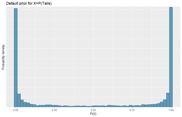
Note that, because of the transformation, this default prior looks substantially different from what we might expect or want. This specifies that, without seeing the data, we believe that the coin is probably either going to give all heads or all tails with it being very unlikely to be a fair coin.

Flat prior

So, let’s change our prior to ##\log(O(X))=\mathcal{N}(\mu=0,\sigma=1.7)## using the following code:

prior.flat <- stan_glm(End ~ 1, data = dat, family = binomial(link = "logit"),
prior_PD = TRUE, prior_intercept = normal(0,1.7))
prior_summary(prior.flat)
mcmc_hist(prior.flat, transformations = inv_logit, binwidth = 0.02)+
expand_limits(x=c(0.0,1.0)) +
labs(title = "Flat prior for X=P(Tails)", x = "P(X)", y = "Probability density")

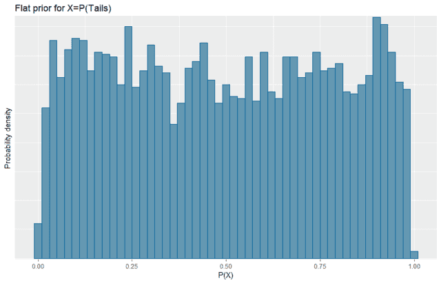
Note that we now have a much more even distribution across the range. This is what we would typically think of as an uninformative prior for this problem. All values of ##P(Tails)## are possible and roughly uniform probability.

Informed prior

Now, realistically, we have seen coins in the past and a decent amount of experience with them. For this study we were given that the coin is a standard US dime, so we know that it is not some trick novelty coin. In our experience, a standard coin might be slightly unfair, but it is close enough to fair that we have not noticed anything despite a lifetime of using such coins.

So let’s choose a prior which reflects that, but is also not overly specific since it is indeed possible that there is some small unfairness that we simply haven’t noticed because we didn’t flip one 40000 times. ##\log(O(X))=\mathcal{N}(\mu=0,\sigma=0.2)## seems to work pretty well. We can implement it as follows:

prior.informed <- stan_glm(End ~ 1, data = dat, family = binomial(link = "logit"),
prior_PD = TRUE, prior_intercept = normal(0,0.2))
prior_summary(prior.informed)

mcmc_hist(prior.informed, transformations = inv_logit, binwidth = 0.02)+
expand_limits(x=c(0.0,1.0)) +
labs(title = "Informed prior for X=P(Tails)", x = "P(X)", y = "Probability density")

prior.informed.df <- as.data.frame(prior.informed)
prior.informed.df$ptails <- inv_logit(prior.informed.df$`(Intercept)`)
ecdf(prior.informed.df$ptails)(0.60)-ecdf(prior.informed.df$ptails)(0.40)
ecdf(prior.informed.df$ptails)(0.51)-ecdf(prior.informed.df$ptails)(0.49)

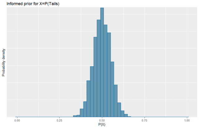
When we plot this, the transformed distribution looks reasonably normal and centered on being fair. This prior has ##P(X\in [0.4,0.6])=0.96## which seems reasonable to expect since we would be surprised to see ##P(Tails)## outside that range, but it isn’t impossible. It also has ##P(X\in [0.49,0.51]) = 0.17## which shows that we are allowing the coin to be practically fair but we are not just assuming that fact or forcing our preconceptions onto the results. So it is a reasonably informed prior but not overly narrow.

Strength of evidence

In Bayesian inference the strength of the evidence, ##P(E|H)/P(E)##, does not dictate our conclusions, but tells us how much we should change our prior beliefs. The data does not “speak for itself”, but it does speak.

##P(E|H)## is called the likelihood, and is very important but is not the only factor that determines the strength of the evidence. Data with a small likelihood can still be strong evidence for a hypothesis provided the data itself has a low probability, i.e. ##P(E)## is small.

In the common setting of comparing two different hypotheses, ##H_A## and ##H_B##, Bayes theorem can be written more conveniently in terms of odds: $$\frac{P(H_A|E)}{P(H_B|E)}=\frac{P(E|H_A)}{P(E|H_B)} \frac{P(H_A)}{P(H_B)} $$  $$O(H_A:H_B|E)=K \ O(H_A:H_B)$$ where ##K=\frac{P(E|H_A)}{P(E|H_B)}## is called the Bayes factor and indicates the relative strength of the evidence for ##H_A## over ##H_B##. In this situation ##P(E)## cancels out.

For our coin flip example the researchers also recorded if the coin started with heads up or tails up. So we can add the starting position into the logistic regression model. Bayes factors depend on the prior, so let’s use the informed prior.

post  <- stan_glm(End ~ Start, data = dat, family = binomial(link = "logit"),
prior_intercept = normal(0,0.2), diagnostic_file = file.path(tempdir(), "post.csv"))
post0 <- stan_glm(End ~    1, data = dat, family = binomial(link = "logit"),
prior_intercept = normal(0,0.2), diagnostic_file = file.path(tempdir(), "post0.csv"))
bayesfactor_models(post, denominator = post0)

In this case ##K=0.161##, which means that there is evidence against the model that the starting position influences ##P(Tails)##. This evidence is very weak, despite the 40000 data points.

Philosophy of science

So now we have seen the basics of Bayes’ theorem and how it applies to statistical inference in the context of scientific studies. But as I mentioned earlier, that is not all; Bayesian statistics automatically enforces the key principles of scientific philosophy. What is notable is that these principles are not put into the process of Bayesian inference by hand, but they emerge naturally and automatically from the mathematical framework itself.

Ockham’s razor

Ockham’s razor is the principle that a scientific model should be as simple as possible in keeping with the data. Of course, sometimes the simplest possible model is still complicated, and this becomes even more difficult to discern when the data itself is uncertain. So how can you systematically decide when a more complicated model is necessary and when a simpler model is preferred?

As we saw in the “Strength of evidence” section, the Bayes factor can be used for this purpose. Since ##K=0.161##, the simpler model is naturally preferred according to Bayes. This contrasts with the frequentist R² which is always larger for the more complicated model. The more complicated model will always [b]fit[/b] the data better, but often the simpler model will [b]predict[/b] the data better and the Bayes factor indicates that.

Simpler models make sharper predictions because they have less “wiggle room”. They have fewer parameters to fine-tune to match arbitrary data. So if the data is inside the region of sharper support, the simpler model is preferred. Outside that region, however, the additional complexity of the complicated model is warranted by the data. Ockham’s razor is used only where it is applicable.

For example, the likelihood of getting ##n## tails out of 40000 flips of a fair coin is given by the binomial distribution ##PMF(B(40000,0.5),n)##. The likelihood of getting ##n## tails out of 40000 flips of a coin with unknown ##P(Tails)## with a uniform prior on possible values of ##P(Tails)## is a flat ##1/40000##. We can plot these two likelihood functions together, their ratio is the Bayes factor.

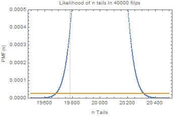
Note the vertical line indicating the actual data. It is within the region where the simpler model is favored, but if hypothetically we had obtained only 19600 Tails out of 40000 then we would have had data that was so unlikely under the simple model that Ockham’s razor would have been rejected. So not only does Bayesian inference automatically apply Ockham’s razor when warranted, it also has a systematic way to reject it when the data warrant its rejection.

Popper’s falsifiability

Popper’s idea of falsification is essentially the idea that no scientific theory can ever be “proven” but they can be “disproven”. In other words, his idea is that contradictory evidence is somehow much stronger than supporting evidence. This indeed can be seen in the Bayes’ factor ##K=\frac{P(E|H_A)}{P(E|H_B)}##.

Consider ##H_A=H## and ##H_B=\neg H##, then ##K=\frac{P(E|H)}{P(E|\neg H)}##. Suppose ##E## is some evidence that is definitively predicted by ##H##, then ##P(E|H)\approx 1##, but for many reasonable hypotheses ##P(E|\neg H)## is not particularly small so ##K## is greater than 1 but not large. In contrast, ##P(\neg E|H)\approx 0## and typically ##P(\neg E|\neg H)## is again not particularly small so in this case ##K\approx 0##. So Bayesian statistics naturally implements the idea that contradictory information is stronger than confirmatory information.

Of course, Popper’s idea of falsification can be overdone. The idea that confirmatory evidence is worthless is too extreme, as evidenced by the fact that Newtonian gravity is still taught and used despite being conclusively falsified. With Bayes’ theorem you can indeed perform verification also, including quantitatively demonstrating support for a null hypothesis. A proper application of Bayesian methods allows a researcher to automatically strike the right balance between the Popper’s correct core idea and its potential over-exaggeration.

Ethics and civic responsibility

The last part of scientific philosophy that I would like to touch on is scientific ethics and civic responsibility. Very few scientists today are running their own experiments using their own funds. Many, possibly most, are funded directly or indirectly by the taxpaying public. The public pays us to gather knowledge, to think deeply, and experiment carefully. We have an ethical obligation to society to respect that trust and ensure that we provide good value for those funds.

One problem with frequentist statistics is the multiple comparisons issue. This issue is well illustrated here:

Basically, if your data has a p=0.05 chance of having arisen by random chance and you do 20 tests then it is likely that one of them will falsely indicate a significant result. To reduce this problem frequentists use a variety of corrections for multiple comparisons, all of which reduce the significance (increase the frequentist p-value) of a result the more tests are performed on the data.

As a result, there is a very strong incentive to limit the number of statistical tests performed on a data set. A researcher who intended to perform as many tests as they could think of would be ensuring that the results would be non-significant after correcting for multiple comparisons. Furthermore, data re-use is impossible since using the data again later would change the p-values of the original study.

The outcome is that data must become disposable under frequentist methods. You use it once and then you must discard it, never to touch it again. This is far more wasteful than failing to recycle your trash because the discarded resource is so expensive and valuable, and far more ethically questionable since the wasteful scientist did not pay for the data that he is throwing away. When there was no other alternative, this could be justified, but given that there is now an alternative, I do not believe that it is ethical to avoid it.

Under Bayesian statistics the multiple comparisons issue disappears. Data can be used, reanalyzed, reused, shared, and so forth. At a minimum previous data should be included in the informed prior of future studies, but Bayesian methods can go beyond that. A Bayesian analysis samples the joint posterior distribution of all parameters, and that posterior can be analyzed as many ways as you like, and it doesn’t change the probability of any previous analyses. The Bayesian approach would naturally detect that the color-based model in the XKCD jellybean experiment above had a lower Bayes factor than the simpler model, regardless of how many colors are tested and without any artificial or external correction factors.

Ideally, data should be archived and shared in an accessible place, particularly data obtained using public funds. We should not willingly and needlessly destroy a valuable and expensive resource, even if it requires us to leave our statistical comfort zone. With Bayesian methods, data can be shared and re-analyzed for other purposes that we did not conceive of, and it can be used to make better priors for the next scientist. In addition to the economic responsibility, research that requires the sacrifice of experimental animals or that exposes human subjects to potential harm (even with informed consent) has a particular ethical obligation to make sure that the most knowledge possible is obtained from the experiment.

Summary

In this post we have covered a lot of scientific topics and discussed the Bayesian approach with its benefits and challenges. We have seen how the various parts of Bayes’ theorem work in the context of science, and with the simple example of the coin flip data. The prior distribution summarizes our current state of knowledge, the Bayes’ factor summarizes the strength of the new evidence, and the posterior summarizes our new state of knowledge after considering the new evidence. Bayesian methods naturally answer the scientific questions that researchers want to know, as well as rigorously following the most important “philosophy of science” principles when and only when they apply. Finally, Bayesian methods allow the reuse of data in a way that must be avoided when using frequentist methods.