Lie Algebras: A Walkthrough The Representations

Part III: Representations

10. Sums and Products.

Frobenius began in ##1896## to generalize Weber’s group characters and soon investigated homomorphisms from finite groups into general linear groups ##GL(V)##, supported by earlier considerations from Dedekind. Representation theory was born, and it developed fast in the following decades. The basic object of interest, however, has never been changed: A structure-preserving mapping from one class of objects into another which allows matrix representations.

Definition: A representation of a (Lie) group G on a vector space ##V## is a (Lie) group homomorphism
\begin{align*}
\varphi\, &: \,G \longrightarrow GL(V)\\
\varphi(x\cdot y)&=\varphi(x)\circ \varphi(y)
\end{align*}
Definition: A representation of a Lie algebra ##\mathfrak{g}## on a vector space ##V## is a Lie algebra homomorphism
\begin{equation}
\begin{aligned}
\varphi\, &: \,\mathfrak{g} \longrightarrow \mathfrak{gl}(V)\\
\varphi([X,Y])&=[\varphi(X),\varphi(Y)]=\varphi(X)\circ \varphi(Y)-\varphi(Y)\circ \varphi(X)
\end{aligned}
\end{equation}
This is called a linear representation of ##\mathfrak{g}## to be exact. Formally it is the pair ##(V,\varphi)##, but usually only one part is referred to as representation, preferably ##\varphi##. If ##V## is finite-dimensional, then the representation is called finite-dimensional, if ##\operatorname{ker}(\varphi)=\{\,0\,\}## then the representation is called faithful – nothing gets lost. A representation is called irreducible, if ##\{\,0\,\}## and ##V## are exactly the only two (under ##\varphi(\mathfrak{g})##) invariant subspaces of ##V##, resp. if the ##\varphi(X)## cannot be written as block matrices ##\begin{bmatrix}A&B\\0&C\end{bmatrix}## with the same block structure simultaneously for all ##X\in \mathfrak{g}##.

Another notation is: ##\mathfrak{g}## operates on ##V##, or ##V## is a ##\mathfrak{g}-##module
\begin{align}
X.v := \varphi(X)(v)
\end{align}
They all are simply different wordings of equation ##(1)##.

Given two representations ##(V,\varphi)## and ##(W,\psi)## of ##\mathfrak{g}## we can define other representations by

\begin{align*}
\text{ direct sum: }\,&(V\oplus W,\varphi \oplus \psi) \, : \,\mathfrak{g} \longrightarrow \mathfrak{gl}(V)\oplus \mathfrak{gl}(W) \subseteq \mathfrak{gl}(V\oplus W)\\\text{as } & (\varphi \oplus \psi)(X)(v+w)=\varphi(X)(v) + \psi(X)(w)\\
&X.(v+w)=X.v +X.w\\
&\\
\text{ tensor product: }\, &(V\otimes W,\varphi \otimes \psi) \, : \,\mathfrak{g} \longrightarrow \mathfrak{gl}(V\otimes W)\\
\text{as } & (\varphi \otimes \psi)(X)(v\otimes w)=\varphi(X)(v)\otimes w + v \otimes \psi(X)(w)\\
&X.(v\otimes w)=X.v \otimes w +v \otimes X.w\\
&\\
\text{ dual: } \,& (V^*,\varphi^*)\, : \,\mathfrak{g}\longrightarrow \mathfrak{gl}(V^*)\\\text{as } & \varphi^*(X)(f) = -f(\varphi(X)(v))\\
&X.f(v)=-f(X.v)
\end{align*}

The similarity in the definition of tensor products to the Leibniz rule is no incident: a differential ##X## operating on a certain product ##v * w##.

The minus sign in the definition on dual spaces is necessary, since otherwise we would get an anti-homomorphism in ##(1)## due to the rule ##f(X.Y.v)=X.f(Y.v)=(X.f)(Y.v)=Y.(X.f(v))\,.##

A representation is called completely reducible, if it can be written as a direct sum of irreducible representations, or equivalently if any invariant subspace ##W\subseteq V## has an invariant complement ##W’ \subseteq V## such that ##V=W\oplus W’.##

Theorem (Weyl): Let ##\mathfrak{g}\subseteq \mathfrak{gl}(V)## be a finite dimensional, semisimple linear Lie algebra, e.g. the simple classical Lie algebras, with finite dimensional vector space ##V##. Then ##\mathfrak{g}## contains the semisimple (diagonal) and nilpotent (upper triangular) parts in ##\mathfrak{gl}(V)## of all its elements.

This theorem has a very important consequence. Let us consider the Jordan decomposition
$$
\operatorname{ad}(X) = \operatorname{ad}(X_s)+\operatorname{ad}(X_n)
$$
Then ##X=X_s+X_n## is called the abstract Jordan decomposition of ##X\in \mathfrak{g}##. Abstract, because as a linear transformation, which ##X\in \mathfrak{g}\subseteq \mathfrak{gl}(V)## is, it already has a usual Jordan decomposition. Now Weyl’s theorem states, that these two decompositions coincide!

Corollary: Let ## \mathfrak{g}## be a finite dimensional, semisimple Lie algebra, and ##(V,\varphi)## a finite dimensional representation of ##\mathfrak{g}##. If ##X=X_s+X_n## is the Jordan decomposition of ##X\in \mathfrak{g}##, then $$\varphi(X)=\varphi(X_s)+\varphi(X_n)$$ is the Jordan decomposition of (the matrix) ##\varphi(X)##.

This might read a bit confusing for the first time. However, Weyl’s theorem says, that we do not have to bother this confusion: there is only one Jordan decomposition, whether as given matrix of one of the classical Lie algebras or as a vector within these Lie algebras where the decomposition is done along ##\operatorname{ad}(X) \in \mathfrak{gl(g)} \subseteq \mathfrak{gl(gl}(V))##.

11. Weights.

Definition: Let ##(V,\varphi)## be a finite dimensional representation of a nilpotent Lie algebra ##\mathfrak{g}##. A linear function ##\lambda \in \mathfrak{g}^*## is called a weight of ##\varphi## if there is a vector ##0\neq v \in V## and an integer ##m=m(v)\geq 1## such that for all ##X\in \mathfrak{g} ##
$$
(\varphi(X)-\lambda \cdot \operatorname{id}_\mathfrak{g})^m(v)=0
$$
In this case the set of all these vectors together with ##0## form a linear subspace $$V_\lambda = \{\,v\in V\,|\,(\varphi(X)-\lambda \cdot \operatorname{id}_\mathfrak{g})^m(v)=0\,\} \subseteq V$$ which is called weight (sub)space of ##\varphi## corresponding to ##\lambda##.

If ##V_\lambda =V## then ##\varphi## is a nil representation called ##\lambda-##representation and $$\lambda(X)\cdot \dim V = \operatorname{tr}(\varphi(X))$$
Given two finite dimensional ##\lambda_i -##representations ##(V_i,\varphi_i)## of ##\mathfrak{g} \, (i=1,2\, ; \,\lambda_i\in \mathfrak{g}^*)## then $$(V_1\otimes V_2,\varphi_1\otimes \varphi_2) \text{ is a } (\lambda_1+\lambda_2)-\text{representation of } \mathfrak{g}$$
Note that in case ##\mathfrak{h}## is a Cartan subalgebra of a semisimple Lie algebra ##\mathfrak{g}##, ##\mathfrak{h}## is toral, thus diagonalizable, thus Abelian, thus a nilpotent Lie algebra, and the weight spaces corresponding to ##(V,\varphi )=(\mathfrak{g},\operatorname{ad}_\mathfrak{h})## are the eigenspaces ##E_\lambda(\mathfrak{h})=V_\lambda ## and therefore precisely the root spaces. In this sense, weight spaces are the generalization of root spaces for arbitrary representations. The particular case of a Cartan subalgebra (with an arbitrary finite-dimensional representation) is still a very important one, especially for the simple Lie algebras ##\mathfrak{su}(n)## which occur in particle and quantum physics.

So the general way to go for simple Lie algebras ##\mathfrak{g}## with a Cartan subalgebra ##\mathfrak{h}## is: Consider the representation ##(\mathfrak{g},\operatorname{ad}_\mathfrak{h})## in order to study the multiplicative structure of ##\mathfrak{g}## by roots, and in a second step consider arbitrary representations ##(V,\varphi)## to study their actions on specific vector spaces by weights.

Theorem: Let be ##\mathfrak{g}## a nilpotent Lie algebra and ##(V,\varphi)## a finite dimensional, complex representation of ##\mathfrak{g}##. Then the weight subspaces of ##\varphi## corresponding to distinct weights ##\lambda_1,\ldots ,\lambda_r## are linearly independent and
\begin{align}
V = \sum_{i=1}^r{} V_{\lambda_i} = \bigoplus_{i=1}^r{} V_{\lambda_i}
\end{align}
The sum is usually written with ##\Sigma ## although it is a direct sum.

12. Casimir elements.

In the previous parts, we have seen that the Killing-form is a powerful tool to investigate semisimple Lie algebras. The Killing-form is the trace form of the adjoint representation. And as weights generalize roots, i.e. represent the step from the adjoint to arbitrary representations, we can also ask, how the Killing-form generalizes. Semisimple Lie algebras are direct sums of simple Lie algebras and their representations split accordingly. Therefore we may consider for the sake of simplicity a simple Lie algebra ##\mathfrak{g}## and a finite-dimensional representation ##(V,\varphi).## Since ##\operatorname{ker}\varphi## is an ideal of ##\mathfrak{g}##, ##V## is either a trivial ##\mathfrak{g}-##module or ##\varphi## is a faithful representation. Let us assume the latter and define the trace form
\begin{align*}
\beta(X,Y) := \operatorname{tr}(\varphi(X)\varphi(Y))
\end{align*}
Then ##\beta## is an associative, symmetric, nondegenerate, bilinear form on ##\mathfrak{g}## and for an ordered basis ##\{\,X_1,\ldots , X_n\,\}## of ##\mathfrak{g}## there is a ##\beta-##dual basis ##\{\,Y_1,\ldots , Y_n\,\}## of ##\mathfrak{g}##, i.e. ##\beta(X_i,Y_j)=\delta_{ij}\,.##
\begin{align*}
c_\varphi = c_\varphi(\beta) := \sum_{i=1}^n\varphi(X_i)\varphi(Y_i)
\end{align*}
is a linear transformation of ##V## which commutes with ##\varphi(\mathfrak{g})##; ##c_\varphi## is called Casimir element of ##\varphi##. We have ##\operatorname{tr}c_\varphi = \dim(\mathfrak{g})## and in case ##\varphi## is irreducible, ##c_\varphi## is a scalar multiplication with ##c_\varphi = \dim(\mathfrak{g})/\dim(V)##.

13. Examples.

The Three Dimensional Simple Lie Algebra.

The (ordered) standard basis ##(X,H,Y)## or sometimes ##(E,H,F)## of the three dimensional simple Lie algebra ##\mathfrak{sl}(2)## is in terms of the Pauli matrices
\begin{equation}
\begin{aligned}
X &= \frac{1}{2} \sigma_1 +\frac{1}{2}\,i\,\sigma_2=\begin{bmatrix}0&1\\0&0\end{bmatrix}\\[6pt]
H &= \sigma_3 = \begin{bmatrix}1&0\\0&-1\end{bmatrix} \\[6pt]
Y &= \frac{1}{2} \sigma_1 -\frac{1}{2}\,i\,\sigma_2=\begin{bmatrix}0&0\\1&0\end{bmatrix}
\end{aligned}
\end{equation}
with the multiplications ##[H,X]=2X\; , \;[H,Y]=-2Y\; , \;[X,Y]=H## from which we get
\begin{align*}
\operatorname{ad}(\alpha,\beta,\gamma)=\operatorname{ad}(\alpha X+\beta H +\gamma Y) = \begin{bmatrix} -2\beta&-2\alpha&0\\-\gamma&0&\alpha\\0&2\gamma&-2\beta\end{bmatrix}\,.
\end{align*}
With the (irreducible) representation ##1=\operatorname{id}\, : \,\mathfrak{sl}(2)\subseteq \mathfrak{gl}(\mathbb{F}^2)## we have a ##\operatorname{id}-##dual basis ##(Y,\frac{1}{2}H,X)## and the Casimir element
\begin{align*}
c_{\operatorname{id}}=XY+\dfrac{1}{2}H^2+YX=\dfrac{3}{2}\cdot \begin{bmatrix}1&0\\0&1\end{bmatrix} = \dfrac{\dim(\mathfrak{sl}(2))}{\dim(\mathbb{F}^2)}\cdot \operatorname{id}_{\mathbb{F}^2}
\end{align*}
The general classification of finite dimensional, irreducible, complex ##\mathfrak{sl}(2,\mathbb{C})## representations ##(V,\varphi)## can be summarized as follows.

Theorem (##\mathfrak{sl}(2,\mathbb{C})## modules / representations):

1. All weights ##\lambda##, i.e. the eigenvalues of the semisimple (diagonizable) operation of ##H## on ##V## are integers and the weight spaces (eigenspaces) ##V_\lambda## of this operation are one dimensional. The highest (maximal) weight be ##m## and a vector ##v_m \in V_m## is called maximal vector or vector of highest weight.
2. ##\displaystyle V = \bigoplus_{\stackrel{k=0}{\lambda=-m+2k}} ^{m}V_{\lambda} = \bigoplus_{\stackrel{k=0}{\lambda=-m+2k}}^{m}\;\{ v\in V\, : \,\varphi(H)(v)=\lambda \cdot v \}##
3. There is up to isomorphisms only one unique finite dimensional, irreducible representation of ##\mathfrak{sl}(2,\mathbb{C})##, resp. ##\mathfrak{su}(2,\mathbb{C})## per dimension of the representation space ##V##.
4. Let ##v_m## be a maximal vector. Then for ##k=0,\ldots , m## we define
   $$
   v_{m-2k-2} := \frac{1}{(k+1)!}\;\varphi(Y)^{k+1}(v_m)\; \text{ and } \;v_{-m-2}=v_{m+2}=0
   $$
   and get the following operation rules
   \begin{equation*}
   \begin{array}{ccc}
   \varphi(X)(v_{m-2k})&=&(m-k+1)\;v_{m-2k+2}\\
   \varphi(H)(v_{m-2k})&=&(m-2k)\;v_{m-2k}\\
   \varphi(Y)(v_{m-2k})&=&(k+1)\;v_{m-2k-2}
   \end{array}
   \end{equation*}
5. If ##(V,\varphi)## is any (not necessarily irreducible) finite-dimensional representation, then the eigenvalues are all integers, and each occurs along with its negative an equal number of times. In any decomposition of ##V## into irreducible submodules, the number of summands is precisely ##\operatorname{dim}V_0 + \operatorname{dim} V_1\,##.

The Adjoint Representation.

A representation consists actually of three parts: What is represented, as what is it represented, and how is it represented? Thus it makes a big difference whether we talk about a representation of a Lie algebra or a representation on a Lie algebra. In case of the adjoint representation, we have both with the same name:

The adjoint representation of a Lie group ##G## on its Lie algebra by conjugation:
\begin{align*}
\operatorname{Ad}\, : \,G &\longrightarrow GL(\mathfrak{g})\\
g &\longmapsto \left(X \longmapsto gXg^{-1} \right)
\end{align*}
and the adjoint representation of a Lie algebra ##\mathfrak{g}## on itself by left (Lie) multiplication:
\begin{align*}
\operatorname{ad}\, : \,\mathfrak{g} &\longrightarrow \mathfrak{gl(g)})\\
X &\longmapsto \left(Y \longmapsto [X,Y] \right)
\end{align*}
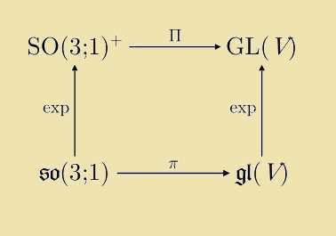
Both adjoint representations are connected by the formula ##(X\in \mathfrak{g})##
\begin{align}
\operatorname{Ad}(\exp X) = \exp(\operatorname{ad}(X))
\end{align}
This formula can be visualized by the commutativity of the following diagram:
\begin{equation*}
\begin{aligned}
G &\stackrel{\operatorname{Ad}}{\longrightarrow} GL(\mathfrak{g}) \\
\exp \uparrow & \quad \quad \uparrow \exp \\
\mathfrak{g} &\stackrel{\operatorname{ad}}{\longrightarrow} \mathfrak{gl(g)}
\end{aligned}
\end{equation*}
between Lie groups (analytic manifolds in which group multiplication and inversion are analytical functions) in the top row and their tangent spaces at ##g=1## (Lie algebras) in the bottom row. It reflects an integration process, similar to the standard ansatz when solving differential equations by assuming an exponential function as solution. In this sense the adjoint representation of the Lie algebra is the differential of the adjoint representation of the Lie group, and the adjoint representation of the Lie group the integrated adjoint representation of the Lie algebra. It integrates ##0\in \mathfrak{g}## to ##1 \in G##, resp. the tangent space at ##g=1## to the connection component of the group identity. The differentiation process can be achieved by considering flows on the manifolds (cp. [6] or [12],[13]).

It can be proven, that given an analytic group homomorphism ##\varphi\, : \,G_1\longrightarrow G_2## between two Lie groups with the differential ##D\varphi##
\begin{align}
\operatorname{Ad}(\varphi(g)) \circ D\varphi = D\varphi \circ \operatorname{Ad}(g) \quad (g \in G_1)\,.
\end{align}
Linear transformations generally do not commute, so that the fundamental formula of the exponential function ##e^{a+b}=e^a\cdot e^b## does not apply here. Of course, we still have ##\exp(c\cdot X)=e^c\cdot \exp(X)## for the scalar multiplication, but it is also of interest to know, how the product of two exponentiated Lie algebra vectors behave with respect to other Lie algebra vectors.

Theorem (Baker-Campbell-Hausdorff Formula):
\begin{align*}
\exp(X)\cdot \exp(Y) = \exp&\left(X+Y+\dfrac{1}{2}[X,Y]+\right.\\
&\left. +{\frac {1}{12}}[X,[X,Y]]-{\frac {1}{12}}[Y,[X,Y]]\right.\\
&\left. -{\frac {1}{24}}[Y,[X,[X,Y]]]\right.\\
&\left.-{\frac{1}{720}}([[[[X,Y],Y],Y],Y]+[[[[Y,X],X],X],X])\right.\\
&\left. +{\frac{1}{360}}([[[[X,Y],Y],Y],X]+[[[[Y,X],X],X],Y])\right.\\
&\left. +{\frac {1}{120}}([[[[Y,X],Y],X],Y]+[[[[X,Y],X],Y],X])+\cdots \right)
\end{align*}

The Natural Representation of a Linear Lie Algebra.

A linear Lie algebra is a subalgebra ##\mathfrak{g}\subseteq \mathfrak{gl}(V)## of linear transformations on a vector space ##V##. Thus there is a natural representation ##(V,\operatorname{id})## given by $$\operatorname{id}_\mathfrak{g}(X)(v)=X.v=X\cdot v =X(v)$$
There is a subtlety with the definition here. The natural representation of a linear Lie algebra is only given if the multiplication is defined by its subalgebra property as $$[X,Y](v)=X(Y(v))-Y(X(v))$$ which is normally not especially mentioned. But theoretically, it would be possible, that the Lie multiplication is defined differently, in which case this has to be mentioned. E.g. we could define another, Abelian multiplication on ##\mathfrak{sl}(2,\mathbb{R})\subseteq \mathfrak{gl}(\mathbb{R}^2)## by just setting ##[X,Y]=0##. In this case we have a three-dimensional Euclidean space as Lie algebra, which should be written as ##\mathbb{R}^3## instead. It can also happen, that a definition doesn’t immediately show, that the Lie algebra is isomorphic to a certain linear one. Remember Ado’s theorem that all (real or complex, finite-dimensional) Lie algebras are isomorphic to a linear one. The natural representation is therefore an important representation, not the least because all results from linear algebra immediately apply. Note that a linear Lie group ##G \subseteq GL(V)## and its Lie algebra ##\mathfrak{g}\subseteq \mathfrak{gl}(V)## operate on, resp. are represented as linear transformations of the same vector space ##V##.

The Algorithm Manifold.

Lie multiplication, even if not defined as subsequent application of a linear transformation or other operators is still a bilinear transformation ##\mathfrak{g}\times \mathfrak{g}\longrightarrow \mathfrak{g}## and as such can be written as
\begin{align*}
\beta(X,Y) = [X,Y] = \sum_{i}^r u_i(X)\cdot v_i(Y) \cdot W_i
\end{align*}
with ##(1,2)## tensors ##u_i\otimes v_i \otimes W_i \in \mathfrak{g}^*\otimes\mathfrak{g}^*\otimes\mathfrak{g}## which is called a bilinear algorithm. The set of all bilinear algorithms of ##\beta## builds an affine variety which is called algorithm manifold of ##\beta##. The group
\begin{align*}
\Gamma(\beta)=\left\{\,\varphi^*\otimes \psi^*\otimes \chi^* \in GL(\mathfrak{g}^*\otimes\mathfrak{g}^*\otimes\mathfrak{g})\,:\,[X,Y]=\chi\left([\varphi(X),\psi(Y)]\right)\,\right\}
\end{align*}
is called isotropy group of ##\beta## and is an example of a group operation on ##\mathfrak{g}^*\otimes\mathfrak{g}^*\otimes\mathfrak{g}##. The Lie algebras here serve as representation space and the group elements are those which leave the Lie multiplication invariant, esp. its tensor rank ##r##. With the embedding ##\alpha^{-1}\longmapsto \alpha^*\otimes \alpha^*\otimes \alpha^{-1}## we have group monomorphism from ##\operatorname{Aut(\mathfrak{g})} \longrightarrow \Gamma(\mathfrak{g}).## It can be shown that for simple Lie algebras (as well as for their Borel subalgebras) the automorphisms are the only elements of the isotropy group with the exception that
$$
\Gamma(\mathfrak{sl}(2,\mathbb{F})) \cong GL(SL(2,\mathbb{F}))/\mathbb{F}^*
$$
This means an exception for the tangent space of the unitary group ##SU(2),## too, since ##\mathfrak{su(2)\cong \mathfrak{sl}(2)}##. In other words: Due to its minimality (cp. its Dynkin diagram “##\circ ##”), the three-dimensional simple Lie algebra behaves a little bit differently than other simple Lie algebras.

A Related Lie Algebra as Representation.

The investigation of the isotropy group leads to the consideration of transposable transformations for which ##[\tau(X),Y]=[X,\tau^\dagger(Y)]##, and with the standard split ##\tau =\frac{1}{2}(\tau+\tau^\dagger)+\frac{1}{2}(\tau – \tau^\dagger)## into a symmetric ##[(\tau+\tau^\dagger)(X),Y]=[X,(\tau+\tau^\dagger)(Y)]## and an antisymmetric part ##(\tau-\tau^\dagger)## to
$$
A(\mathfrak{g}) = \{\,\alpha \in \mathfrak{gl}(\mathfrak{g})\,:\,[\alpha(X),Y]=-[X,\alpha(Y)]\text{ for all }X\in \mathfrak{g}\,\}
$$
which turns out to be a Lie algebra again, the Lie algebra of antisymmetric transformations of ##\mathfrak{g}##. As always with such definitions, the question of existence has to be answered, or more precisely, whether ##A(\mathfrak{g})## can be different from the zero Lie algebra. The trivial case is of course when ##\mathfrak{g}## is Abelian, in which case ##A(\mathfrak{g})=\mathfrak{gl(g)}##. On the other hand, it can be shown that indeed ##A(\mathfrak{g})=\{\,0\,\}## whenever ##\mathfrak{g}## is a simple Lie algebra. However ##\mathfrak{gl(g)} \supsetneq A(\mathfrak{g})\neq \{\,0\,\}## for any solvable, non Abelian Lie algebra as e.g. the Borel subalgebras of simple Lie algebras:

Let ##\mathfrak{g}## be a finite dimensional complex, non Abelian Lie algebra. By Lie’s theorem there is a one dimensional ideal ##\mathfrak{I}=\langle I \rangle \subseteq \mathfrak{g}##, hence ##[X,I]=\lambda(X)I## for some ##\mathfrak{g}^* \ni \lambda \neq 0 ##. With ##\alpha(X):=\lambda(X)I## we get a non trivial antisymmetric transformation.

In a way the antisymmetric Lie algebra ##A(\mathfrak{g})## measures the point where ##\mathfrak{g}## lies between simple (most structured) and Abelian (least structured) Lie algebras. The transformation defined above is by the way the only one for Borel subalgebras of simple Lie algebras (with the exception of ##\mathfrak{sl}(2)##). So the less structure ##\mathfrak{g}## has, the more structure has ##A(\mathfrak{g})## and vice versa.

Theorem (Antisymmetric Transformations): ##A(\mathfrak{g})## is a ##\mathfrak{g}-##module, i.e.
\begin{equation}
\begin{aligned}
\mathfrak{g}&\longrightarrow \mathfrak{gl(A(\mathfrak{g}))}\\
X&\longmapsto \left(\alpha \longmapsto [\operatorname{ad}(X),\alpha]=\operatorname{ad}(X)\circ \alpha -\alpha \circ \operatorname{ad}(X)\right)
\end{aligned}
\end{equation}
defines a representation of ##\mathfrak{g}## on ##A(\mathfrak{g})##.

This follows from repeated applications of the Jacobi identity and the definition of an antisymmetric transformation. Since ##A(\mathfrak{g})## is again a Lie algebra, we can ask for ##A(A(\mathfrak{g})), A(A(A(\mathfrak{g})))## etc. or build the semidirect product ##\mathfrak{g}\ltimes A(\mathfrak{g})## and then repeat the process. Even
$$
[X,Y]\longmapsto \alpha([X,Y])
$$
with a fixed antisymmetric transformation ##\alpha\in A(\mathfrak{g})## defines again a Lie algebra structure on the same vector space ##\mathfrak{g}##. In this sense, the antisymmetric transformations build a large pool of possible representations.

Differential Operators.

Lie algebras and differential operators are closely related in the sense that a set of differential operators can build the basis for a Lie algebra that operates on some Hilbert space, i.e. in general infinite-dimensional representation spaces.
E.g. we define ##D_n :=x^n\cdot \dfrac{d}{dx}\quad (n \in \mathbb{Z})##, then $$[D_n,D_m]=(m-n)D_{n+m-1}$$ The Lie algebra generated by these differential operators is infinite-dimensional and operates on the Hilbert space of smooth real functions ##C^\infty(\mathbb{R})##. We get a finite dimensional example with
\begin{align*}
\mathfrak{g} \longrightarrow &\mathfrak{gl}(C^\infty(\mathbb{R})) \\[6pt]
\mathfrak{g} :=&\langle D_{-n+1},D_1,D_{n+1} \rangle \\[6pt]
&D_{-n+1}(f)=x^{-n+1}f\,’\, , \,D_1(f)=x f\,’\, , \,D_{n+1}=x^{n+1}f\,’\\[6pt]
&[D_{-n+1},D_1]=nD_{-n+1}\, , \,[D_{-n+1},D_{n+1}]=2nD_1\, , \,[D_1,D_{n+1}]=nD_{n+1}
\end{align*}
which is the three dimensional simple Lie algebra, an isomorphic copy of ##\mathfrak{sl}(2,\mathbb{R})##.

Another example which also operates on ##V=C^\infty(\mathbb{R})## is given by
$$
X_0=\dfrac{1}{2}\left(\dfrac{d^2}{dx^2}+x^2\cdot \operatorname{id}_V \right)\, , \,X_1=\dfrac{d}{dx}\, , \,X_2=x\cdot \operatorname{id}_V\, , \,X_3=\operatorname{id}_V
$$
which yields the non zero multiplications
$$
[X_1,X_2]=X_3\, , \,[X_0,X_1]=-X_2\, , \,[X_0,X_2]=X_1
$$
It is a four dimensional, solvable, real Lie algebra called oscillator algebra. It has a central element ##X_3## and with ##\langle X_1,X_2,X_3 \rangle## a copy of the Heisenberg algebra as nilradical ##\mathfrak{H}=[\mathfrak{g},\mathfrak{g}]##, and ##\mathfrak{h}=\langle X_0,X_3\rangle## as Cartan subalgebra: $$\mathfrak{h}\subsetneq\mathfrak{g}=\mathfrak{H}\rtimes \mathbb{R}\cdot X_0\,.$$

14. Epilogue

I hope I could have shown how rich and complex the world of Lie algebra representations is. For further investigations in this area, I recommend the sources ##[18],[19],[20]## and the literature quoted therein. Other interesting keywords to search for are: quasi-exact solvability, Schrödinger operator, oscillator algebra, the realization of the Lie algebra, Lie algebra of differential operators, highest weights.