Learn Lie Algebras: A Walkthrough The Structures

Part II: Structures

5. Decompositions.

Lie algebra theory is to a large extend the classification of the semisimple Lie algebras which are direct sums of the simple algebras listed in the previous paragraph, i.e. to show that those are all simple Lie algebras there are. Their counterpart are solvable Lie algebras, e.g. the Heisenberg algebra ##\mathfrak{H}=\langle X,Y,Z\,:\, [X,Y]=Z\rangle\,.## They have less structure each and are less structured as a whole as well. In physics, they don’t play such a prominent role as simple Lie algebras do, although the reader might have recognized, that e.g. the Poincaré algebra – the tangent space of the Poincaré group at its identity matrix – wasn’t among the simple ones. It isn’t among the solvable Lie algebras either like ##\mathfrak{H}## is, so what is it then? It is the tangent space of the Lorentz group plus translations: something orthogonal plus something Abelian (solvable).

Theorem: The radical ##\mathfrak{R(g)}## of a Lie algebra ##\mathfrak{g}## is a solvable ideal, ##\mathfrak{g}/ \mathfrak{R(g)} \cong \mathfrak{g}_s \leq \mathfrak{g} ## a semisimple subalgebra and ##\mathfrak{g}## the semidirect product
\begin{align*}
\mathfrak{g} = \mathfrak{R(g)} \rtimes \mathfrak{g}_s \cong \mathfrak{R(g)} \rtimes \mathfrak{g}/\mathfrak{R(g)} \quad (2)
\end{align*}
This decomposition is one of the reasons why semisimple and solvable Lie algebras are of interest. The classification of the former is done, the one on the solvable part unfortunately is not. This is mainly due to the different complexity of their multiplicative structures, resp. the lack of it, or the different complexity of their representations if you like.

The starting point of any classification is usually the question:

What does it consist of and what is it composed of?

We already know that we may consider the elements of a Lie algebra as linear transformations. This is not really astonishing, as we always have ##\operatorname{ad}(\mathfrak{g}) \subseteq \mathfrak{gl}(g)## which are linear transformations, inner derivations to be exact. $$\operatorname{ker}\operatorname{ad}=\mathfrak{Z}(g)$$ is an ideal, which means ##\mathfrak{Z}(g)=0## for semisimple Lie algebras, we even have a faithful (injective) representation as linear transformations for (semi-)simple Lie algebras for free. It also implies, that there is no single Lie algebra element in a semisimple Lie algebra, which commutes with all other elements! Nevertheless, commutation is a convenient property, e.g. simultaneously diagonalizable linear transformations commute.

On the level of linear transformations, the terms diagonalizable, semisimple and toral mean practically the same – at least if all eigenvalues are available, i.e. over algebraically closed fields like ##\mathbb{C}##.

\begin{array}{l|l|l}
\text{property}&\text{applies to}& \text{means} \\
\hline &&\\
\text{semisimple}&\text{linear transformations} & \text{all roots of its minimal} \\ &&\text{polynomial are distinct} \\
\hline &&\\
\text{diagonalizable} & \text{matrices} & \text{there is a basis of eigenvectors}\\
\hline &&\\
\text{toral} & \text{subalgebra of} &\text{all elements are semisimple}\\
&\text{linear transformations} & \\
\hline
\end{array}

The classification of semisimple Lie algebras is based on four fundamental insights. We already mentioned that semisimple Lie algebras are a direct sum of simple Lie algebras and vice versa (1). This result isn’t the first one in its natural order. In fact, one starts with the second from the following list, but this isn’t important in our context:

1. ##\mathfrak{g} = \bigoplus_{i=1}^n \mathfrak{g}_i\quad ##(##\mathfrak{g}## semisimple, ##\mathfrak{g}_i## simple)
2. The Jordan normal form applied on inner derivations.
3. The Cartan subalgebras are toral.
4. The Killing-form defines angles.

Of course, there are a lot of technical details to get there as well as to combine these results to a theory of semisimple Lie algebras, especially some geometrical considerations now that we have angles. However, this basically is it.

The decomposition into simple ideals is extremely helpful, as all inner derivations (##\operatorname{ad}X##) have a block form, and for the Cartan subalgebras, we get a corresponding decomposition ##\mathfrak{h} = \bigoplus_{i=1}^n \mathfrak{h}_i## into the separate Cartan subalgebras, which allows us to concentrate on simple Lie algebras only.

The Jordan normal form is the starting point. As mentioned, this is quite natural as the inner derivations ##\operatorname{ad}X## provide a faithful representation for simple Lie algebras which have no proper ideals, and especially no center.

The Jordan normal form is an additive decomposition of linear transformations in a semisimple (diagonal) part with its eigenvalues and a nilpotent (upper triangular) part. The algebraic multiplicity ##k## of an eigenvalue is its multiplicity in the characteristic polynomial and the dimension of the generalized eigenspace
$$G_\lambda(X)=\operatorname{ker}\,(\operatorname{ad}X -\lambda \cdot \operatorname{id}_\mathfrak{g})^k=\{\,Y\in \mathfrak{g}\,|\,(\operatorname{ad}(X)-\lambda \cdot \operatorname{id}_\mathfrak{g})^k(Y)=0\,\}$$
It is important to distinguish the characteristic, and the minimal polynomial, as well as the geometric multiplicity of an eigenvalue, which is the dimension of the eigenspace
$$E_\lambda(X)=\operatorname{ker}\,(\operatorname{ad}X -\lambda \cdot \operatorname{id}_\mathfrak{g})=\{\,Y\in \mathfrak{g}\,|\,(\operatorname{ad}(X)-\lambda \cdot \operatorname{id}_\mathfrak{g})(Y)=0\,\}\subseteq G_\lambda(X)$$
The geometric multiplicity determines the number of Jordan blocks of the Jordan normal form, the algebraic multiplicity determines the degree of nilpotency of the nilpotent part of a Jordan block, i.e. the number of ones in the upper triangular part of the Jordan normal form.

Theorem (Jordan-Chevalley Decomposition): Let ##V## be a finite dimensional vector space over a field ##\mathbb{F}## and ##\varphi\, : \,V \longrightarrow V## an endomorphism. Then there exist unique endomorphisms ##\varphi_s\; , \;\varphi_n## such that
\begin{align*}\varphi &= \varphi_s+\varphi_n\\  &\varphi_s \text{ is semisimple }\; , \;\varphi_n\text{ is nilpotent }\; , \;[\varphi_s,\varphi_n]=0\\  \varphi_s&=p(\varphi)\; , \;\varphi_n=q(\varphi)\\  &\text{ for some }p(x),q(x) \in \mathbb{F}[x] \text{ with } \,x\,|\,p(x),q(x)
\end{align*}

In particular, ##\varphi_s## and ##\varphi_n## commute with any endomorphism commuting with ##\varphi.## The decomposition ##\varphi=\varphi_s+\varphi_n## is called the additive Jordan-Chevalley decomposition of ##\varphi## and ##\varphi_s,\varphi_n## are called respectively the semisimple and nilpotent part of ##\varphi.## Moreover,
$$
\operatorname{ad}\varphi = \operatorname{ad}\varphi_s +\operatorname{ad}\varphi_n
$$
is the Jordan-Chevalley decomposition of ##\operatorname{ad}\varphi\,.##

The semisimple parts play a key role in the classification of semisimple Lie algebras as well as in their representations. Since they are diagonalizable, i.e. there is a basis of eigenvalues, they also play a key role in physics. Another example of the importance of diagonalizable parts is the following theorem.

Theorem (Malcev Decomposition): A solvable, complex Lie algebra ##\mathfrak{g}## can be written as semidirect product
\begin{align*}
\mathfrak{g} = \mathfrak{R(g)} = \mathfrak{T} \ltimes \mathfrak{N(g)} \quad (3)
\end{align*}
of a toral subalgebra ##\mathfrak{T}## and its nilradical ##\mathfrak{N(g)}.##

Summary: Let ##\mathfrak{g}## be any finite dimensional, complex Lie algebra, then
\begin{align*}
\underbrace{\underbrace{\mathfrak{gl}(V) \supseteq \mathfrak{g}}_{\text{linear Lie algebra}}}_{\text{Theorem of Ado}} = \underbrace{\left( \underbrace{\mathfrak{N(g)}}_{\text{nilpotent}} \rtimes^{(3)} \underbrace{\mathfrak{T}}_{\text{toral}} \right)}_{\text{Theorem of Malcev}} \rtimes^{(2)} \underbrace{\left( \bigoplus_{i=1}^m \underbrace{\mathfrak{g_i}}_{\text{simple}} \right)^{(1)}}_{\text{semisimple}}
\end{align*}

This means, that we now have to decompose the simple Lie algebras, i.e. those with no proper ideals. Again the toral parts are the key to the next decomposition.

Let us assume ##\mathfrak{g}## is a finite-dimensional, complex, simple Lie algebra and ##\mathfrak{h} \subseteq \mathfrak{g}## a Cartan subalgebra (CSA), i.e. a nilpotent and self-normalizing subalgebra. This apparently weird definition of a Cartan subalgebra turns out to be sufficient to derive the following nice properties.

Theorem (CSA):

• Cartan subalgebras are precisely the maximal toral subalgebras.
• Toral subalgebras are Abelian.
• A Cartan subalgebra ##\mathfrak{h}\subseteq \mathfrak{g}## is self-centralizing:
  ##C_\mathfrak{g}(\mathfrak{h})=\{\,X\in \mathfrak{g}\,|\,[X,\mathfrak{h}]=0\,\}=E_0(\mathfrak{h})=\mathfrak{h}##
• ##\operatorname{ad}(\mathfrak{h})## is simultaneously diagonalizable.
• All Cartan subalgebras are conjugate under inner automorphisms of ##\mathfrak{g}##, the group generated by all ##\exp (\operatorname{ad}X)## with ##X\in \mathfrak{g}## ad-nilpotent.

So why isn’t ##\mathfrak{h}## defined as a toral subalgebra in the first place? One reason is, that we haven’t shown the existence of Cartan subalgebras, and this can easier be done with the given definition. Anyway, we get a useful and central

Theorem (Cartan decomposition or Root Space Decomposition):
Let ##\mathfrak{g}## be a (semi)simple Lie algebra and ##\mathfrak{h}\subseteq \mathfrak{g}## a Cartan subalgebra. Then
\begin{align*}
\mathfrak{g} = \mathfrak{h} \oplus \sum_{\alpha \in \Phi}\mathfrak{g}_\alpha \quad (4)
\end{align*}
where ##\mathfrak{g}_\alpha = \{\,X\in \mathfrak{g}\,|\,[H,X]=\alpha(H)X \text{ for all }H \in \mathfrak{h}\,\}## and ##\mathfrak{h}=C_\mathfrak{g}(\mathfrak{h})=\mathfrak{g}_0## are the eigenspaces of all (simultaneously diagonalizable) linear transformations ##\operatorname{ad}H\, , \,\alpha \in \mathfrak{h}^*.##

Those linear forms ##\alpha \neq 0## for which ##\mathfrak{g}_\alpha \neq \{\,0\,\}## are called roots and ##\Phi## the root space of ##\mathfrak{h}##.

All ##\mathfrak{g}_\alpha \,(\alpha \neq 0)## are one dimensional, so let ##E_\alpha## be basis vectors. In particular, we have
\begin{align*}
[H,E_\alpha] = \alpha(H)\cdot E_\alpha \text{ for all }H \in \mathfrak{h}\; , \;\alpha \in \Phi \subseteq \mathfrak{h}^* \quad (5)
\end{align*}

6. Geometry.

What happens next is not less than a little miracle! We will see that the root space of a simple Lie algebra has some unexpected properties, which in the end enabled their classification. Something which is for solvable, and therewith arbitrary Lie algebras far from being achieved. Remember, that this includes examples like the Heisenberg and Poincaré algebra. The best we have for solvable Lie algebras over algebraically closed fields is that they stabilize flags:

Theroem (solvable Lie Algebras): Let ##\mathfrak{g}## be a solvable complex Lie algebra, ##V## an ##n-##dimensional vector space, and ##\varphi\, : \,\mathfrak{g} \longrightarrow \mathfrak{gl}(V)## a Lie algebra homomorphism. Then there is a sequence of subspaces
$$
\{\,0\,\} \subsetneq V_1 \subsetneq \ldots \subsetneq V_n = V
$$
such that ##\dim V_k=k## and ##\varphi(\mathfrak{g})(V_k)\subseteq V_k\,.##
This means especially for the left-multiplication ##\varphi = \operatorname{ad}## that we have a sequence of ideals ##\mathfrak{I}_k \leq \mathfrak{g}## with ##\dim \mathfrak{I}_k=k## and
\begin{align*}
\{\,0\,\} \lneq \mathfrak{I}_1 \lneq \ldots \lneq \mathfrak{I}_m = \mathfrak{R(g)} = \mathfrak{g} \quad (6)
\end{align*}

We now assume that ##\mathfrak{g}## is always a simple finite-dimensional Lie algebra and ##\mathfrak{h}\subseteq \mathfrak{g}## a Cartan subalgebra. The reader may think of it as one of the classical, simple Lie algebras listed in chapter ##3##. Our next task will be to investigate these root spaces ##\mathfrak{g_\alpha}=\operatorname{span}(E_\alpha)##. E.g. the Jacobi identity and equation ##(5)## yield
\begin{align*}
[H,[E_\alpha,E_\beta]]&=[E_\alpha,[H,E_\beta]] – [E_\beta,[H,E_\alpha]]\\
&=\beta(H)\cdot [E_\alpha,E_\beta] -\alpha(H)\cdot [E_\beta,E_\alpha]\\
&=(\alpha+\beta)(H) \cdot [E_\alpha,E_\beta]
\end{align*}
and thus
\begin{align*}
[E_\alpha,E_\beta] \in \mathbb{F}\cdot E_{\alpha+\beta} \quad (7) \end{align*}
and the ladder operators almost shine through.

Next, the Killing-form comes into play. It can be shown that the Killing-form is nondegenerate if and only if ##\mathfrak{g}## is semisimple, i.e.
$$\{\,X\in \mathfrak{g}\,|\,K(X,Y)=\operatorname{tr}(\operatorname{ad}X\circ \operatorname{ad}Y)=0 \text{ for all }Y\in \mathfrak{g})\,\}=\{\,0\,\}
$$
Furthermore, the Killing-form restricted on ##\mathfrak{h}\times \mathfrak{h}## is nondegenerate, and ##K(E_\alpha,E_\beta)=0## for all ##\alpha,\beta \in \mathfrak{h}^* ## with ##\alpha+\beta \neq 0\,;## in particular ##K(\mathfrak{h},E_\alpha)=0\,.##

These are a very strong properties, because it allows us to use certain numbers ##K(H,H’)## as scaling factors while large parts are orthogonal with respect to the Killing-form. We first define a correspondence
\begin{align*}
\mathfrak{h}^* \supset \Phi \longleftrightarrow \{\,F_\alpha\,:\,\alpha\in \Phi\,\} \subset \mathfrak{h} \,\,\text{ by }\,\, \alpha(H)=: K(F_\alpha,H)\; , \;H\in \mathfrak{h} \quad (8)
\end{align*}
define on ##\mathfrak{h}^*## the inner product
\begin{align*}
(\alpha,\beta) := K(F_\alpha,F_\beta)
\end{align*}
and normalize ##H_\alpha := \dfrac{2 \cdot F_\alpha}{(\alpha,\alpha)}## such that equation ##(5)## now reads
\begin{align*}
[H_\alpha,E_\alpha] = \alpha(H_\alpha)\cdot E_\alpha = \dfrac{2}{(\alpha,\alpha)}\cdot \alpha(F_\alpha)\cdot E_\alpha =2\cdot E_\alpha \quad (9)
\end{align*}
Meanwhile our Lie algebra can be written (as a direct sum of vector spaces)
\begin{align*}
\mathfrak{g}= \mathfrak{h} \oplus \sum_{\alpha \in \Phi} \mathfrak{g}_\alpha = \operatorname{span}\{H_\alpha\,|\, \alpha \in \Phi\} \oplus \sum_{\alpha \in \Phi}\mathbb{F}\cdot E_\alpha \quad (10)
\end{align*}
and we already know, that the Cartan subalgebra ##\mathfrak{h}## is Abelian, the one-dimensional eigenspaces ##\mathfrak{g}_\alpha## are simultaneous eigenvectors of the left multiplications ##\operatorname{ad}(H)(X)=[H,X]##, two eigenspaces are Killing orthogonal for ##\alpha +\beta \neq 0##, and that ##\mathfrak{h}## is spanned by vectors ##H_\alpha## which satisfy equation ##(9)##.  The miracle can be summarized in the following theorem, and especially the third property is essential for what follows.

Theorem (Root System): Let ##\alpha , \beta \in \Phi## be roots such that ##\alpha + \beta \neq 0\,.##

1. ##0 \notin \Phi## is finite and spans ##\mathfrak{h}^*.##
2. If ##\alpha \in \Phi## then ##-\alpha \in \Phi## and no other multiple is.
3. If ##\alpha,\beta \in \Phi ## then ##\langle\beta,\alpha \rangle :=\dfrac{2(\beta,\alpha)}{(\alpha,\alpha)} \in \mathbb{Z}##, the Cartan integers.
4. If ##\alpha,\beta \in \Phi ## then the reflection ##\sigma_\alpha(\beta):=\beta – \dfrac{2(\beta,\alpha)}{(\alpha,\alpha)} \cdot \alpha \in \Phi\,.##

Remarks:

1. ##H_\alpha \triangleq \begin{pmatrix}1&0\\0&-1\end{pmatrix}\; , \;E_\alpha \triangleq \begin{pmatrix}0&1\\0&0\end{pmatrix}\; , \;E_{-\alpha}\triangleq \begin{pmatrix}0&0\\1&0\end{pmatrix}\text{ for }\alpha \in \Phi##
   build simple subalgebras ##\mathfrak{sl}(2)## of type ##A_1##
   $$[H_\alpha,E_\alpha]=2E_\alpha\; , \;[H_\alpha,E_{-\alpha}]=-2E_{-\alpha}\; , \;[E_\alpha,E_{-\alpha}]=H_\alpha\,.$$
2. ##(\alpha,\beta) \in \mathbb{Q}## is a positive definite, symmetric bilinear form, in other words, an inner product on the real vector space ##\mathcal{E}## spanned by ##\Phi##.
3. ##\dim \mathcal{E}= l = \dim \mathfrak{h}^* = \dim \mathfrak{h}= \operatorname{rank}\Phi##

At this point we have all ingredients which are necessary: A real Euclidean vector space ##\mathcal{E}## with an inner product ##(\; , \;)##, reflections ##\sigma_\alpha## relative to the hyperplane ##\mathcal{P}_\alpha=\{\,\beta \in \mathcal{E}\,|\,(\beta,\alpha)=0\,\}##, and most of all, integer values for ##\langle \beta,\alpha \rangle ,## which by the way is only linear in the first argument. However, we can define angles now:
\begin{align*}
&\cos \theta = \cos \measuredangle (\alpha,\beta) := \dfrac{(\alpha,\beta)}{||\alpha||\cdot ||\beta||}=\dfrac{(\alpha,\beta)}{\sqrt{(\alpha,\alpha)}\sqrt{(\beta,\beta)}} \quad (11)\\&\\ &\langle \alpha,\beta\rangle \cdot \langle \beta,\alpha \rangle = 4\cos^2 \theta \in \mathbb{N}_0 \quad (12)
\end{align*}
and we have reduced the classification problem to a geometric problem! What’s left is a discussion of equation ##(12).## Note that the major condition to proceed this way was the equivalence of a nondegenerate Killing-form to a direct sum of simple Lie algebras.

We also know already, that for ##l=1## there is only one possibility ##\Phi = \{-\alpha,\alpha\}##: the simple Lie algebra ##\mathfrak{sl}(2)## of type ##A_1\,.##

7. Dynkin Diagrams.

The hyperplanes ##\mathcal{P}_\alpha \,(\alpha\in \Phi)## partition ##\mathcal{E}## into finitely many regions; the connected components of ##\mathcal{E}-\cup_{\alpha \in\Phi}\mathcal{P}_\alpha## which are called the (open) Weyl chambers. The group generated by the reflections ##\sigma_\alpha\,(\alpha\in\Phi)## is called Weyl group ##\mathcal{W}## of ##\Phi\,.##

Let’s have a look on ##\mathcal{E}=\operatorname{span}\{\Phi\}## and choose a basis ##\Delta =\{\,\alpha_1,\ldots ,\alpha_l\,\}## such that all ##\beta \in \Phi## can be written as ##\beta = \sum_{\alpha \in \Delta}k_\alpha \alpha## with integer coefficients ##k_\alpha##. This can be done such that either all coefficients are positive, in which case we call the root positive ##\beta \succ 0##, or all coefficients are negative, in which case we call the root negative ##\beta \prec 0##, and write ##\Phi = \Phi^+ \cup \Phi^-.## The roots ##\alpha \in \Delta## are called simple, and ##\operatorname{ht}(\beta)=\sum_{\alpha\in \Delta}k_\alpha## the height of ##\beta \in \Phi\,.## A root system ##\Phi## is called irreducible if it cannot be partitioned into two proper orthogonal subsets. Irreducible root systems correspond to simple Lie algebras, i.e. by our assumption that ##\mathfrak{g}## is simple, our root system is irreducible. It can be shown that for an irreducible root system ##\Phi## at most two different root lengths can occur and roots of equal length are conjugate under ##\mathcal{W}##. In the case of two different lengths, we speak of short roots and long roots, in case of only one root length, it’s called long as a convention.

Meanwhile our simple Lie algebra looks like
\begin{align*}
\mathfrak{g} &= \underbrace{\mathfrak{h}\oplus \sum_{\alpha \in \Phi^+ }\mathbb{F}\cdot E_\alpha}_{\text{solvable Borel subalgebra}} \oplus \underbrace{\sum_{\alpha \in \Phi^-} \mathbb{F}\cdot E_\alpha}_{\text{nilpotent subalgebra}} \quad \quad (13) \\[8pt]
\Phi &= \operatorname{span}_\mathbb{Z}\Delta= \operatorname{span}_\mathbb{Z}\{\,\alpha_1,\ldots ,\alpha_l\,\}=\underbrace{ \Phi^+ \,\cup\,\Phi^-}_{\text{partially ordered}} \quad (14)
\end{align*}
Let’s fix an ordering of simple roots ##\Delta = \{\,\alpha_1,\ldots ,\alpha_l\,\}.## Then the matrix of Cartan integers ##(\langle \alpha_i,\alpha_j\rangle)_{i,j}## is called the Cartan matrix of ##\mathfrak{g}\,.##

For distinct positive roots ##\alpha,\beta##, we have
$$
\langle \alpha,\beta \rangle \cdot \langle \beta,\alpha \rangle \in \{\,0,1
,2,3\,\}
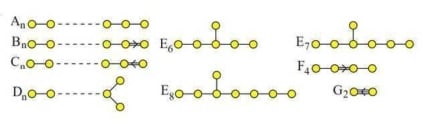
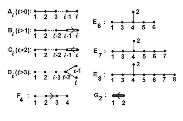
$$
so we can define the Coxeter graph of ##\Phi## to be a graph with ##|\Delta |=l## vertices and the ##i-##th is joined to the ##j-##th ##(i\neq j)## by ##\langle \alpha_i,\alpha_j \rangle \cdot \langle \alpha_j,\alpha_i \rangle## many edges. The Coxeter graph completely determines the Weyl group, but it fails to show us in the case of two or three edges, which vertex of a pair corresponds to a short simple root and which to a long root. Therefore we add an arrow pointing to the shorter of two roots, whenever there is a double or triple edge. The resulting graph is called Dynkin diagram of ##\mathfrak{g}## and allows to recover the Cartan matrix. Irreducible root systems have connected Dynkin diagrams.

Classification Theorem. If ##\mathfrak{g}## is a simple Lie Algebra with an irreducible root system of ##\operatorname{rank} \Phi = \dim \mathfrak{h}=l\,,## then it has one of the following Dynkin diagrams:

8. Cartan Matrices.

\begin{align*}
A_l &: &\begin{pmatrix}2&-1&0&&& \cdots &&0 \\
-1&2&-1&0&&\cdots &&0\\
0&-1&2&-1&0&\cdots&&0\\
\cdot&\cdot&\cdot&\cdot&\cdot&\cdots &\cdot&\cdot\\
0&0&0&0&0&\cdots&-1&2
\end{pmatrix}\\
\\
\hline &&\\
B_l &: &\begin{pmatrix}2&-1&0&&\cdots&&&0\\
-1&2&-1&0&\cdots&&&0\\
\cdot&\cdot&\cdot&\cdot&\cdots&\cdot&\cdot&\cdot\\
0&0&0&0&\cdots&-1&2&-2\\
0&0&0&0&\cdots&0&-1&2
\end{pmatrix}\\
\\
\hline &&\\
C_l &: &\begin{pmatrix}2&-1&0&&\cdots&&&0\\
-1&2&-1&&\cdots&&&0\\
0&-1&2&-1&\cdots&&&0\\
\cdot&\cdot&\cdot&\cdot&\cdots&\cdot&\cdot&\cdot\\
0&0&0&0&\cdots&-1&2&-1\\
0&0&0&0&\cdots&0&-2&2
\end{pmatrix}\\
\\
\hline &&\\
D_l &: &\begin{pmatrix}2&-1&0&\cdot&\cdot&\cdot&\cdot&\cdot&\cdot&0\\
-1&2&-1&\cdot&\cdot&\cdot&\cdot&\cdot&\cdot&0\\
\cdot&\cdot&\cdot&\cdot&\cdot&\cdot&\cdot&\cdot&\cdot&\cdot\\
0&0&\cdot&\cdot&\cdot&-1&2&-1&0&0\\
0&0&\cdot&\cdot&\cdot&\cdot&-1&2&-1&-1\\
0&0&\cdot&\cdot&\cdot&\cdot&0&-1&2&0\\
0&0&\cdot&\cdot&\cdot&\cdot&0&-1&0&2
\end{pmatrix}\\
\\
\hline &&
\end{align*}
\begin{align*}
E_6 &: &\begin{pmatrix}2&0&-1&0&0&0\\
0&2&0&-1&0&0\\
-1&0&2&-1&0&0\\
0&-1&-1&2&-1&0\\
0&0&0&-1&2&-1\\
0&0&0&0&-1&2
\end{pmatrix}\\
\\
\hline &&\\
E_7 &: &\begin{pmatrix}2&0&-1&0&0&0&0\\
0&2&0&-1&0&0&0\\
-1&0&2&-1&0&0&0\\
0&-1&-1&2&-1&0&0\\
0&0&0&-1&2&-1&0\\
0&0&0&0&-1&2&-1\\
0&0&0&0&0&-1&2
\end{pmatrix}\\
\\
\hline &&\\
E_8 &: &\begin{pmatrix}2&0&-1&0&0&0&0&0\\
0&2&0&-1&0&0&0&0\\
-1&0&2&-1&0&0&0&0\\
0&-1&-1&2&-1&0&0&0\\
0&0&0&-1&2&-1&0&0\\
0&0&0&0&-1&2&-1&0\\
0&0&0&0&0&-1&2&-1\\
0&0&0&0&0&0&-1&2
\end{pmatrix}\\
\\
\hline\\
F_4 &: &\begin{pmatrix}2&-1&0&0\\
-1&2&-2&0\\
0&-1&2&-1\\
0&0&-1&2
\end{pmatrix}\\
\\
\hline &&\\
G_2 &: &\begin{pmatrix}2&-1\\
-3&2
\end{pmatrix}\\
\\
\hline &&
\end{align*}

9. Example.

We will show, how Cartan matrices and root systems can be retrieved from the Dynkin diagram on the example of ##G_2\,.##

The Dynkin diagram tells us that ##\alpha \prec \beta## and ##\langle \alpha,\beta \rangle \langle \beta ,\alpha \rangle=3\,.## The cosine formula tells us, that the angle they enclose is ##30°## but this doesn’t matter here. Since the only ways to get an integer product of three are ##3\cdot 1 = (-3)\cdot (-1)=3## we may assume w.l.o.g. and the sign in the theorem of root systems in mind, that ##\langle \alpha,\beta\rangle = -1## and ##\langle \beta,\alpha\rangle=-3\,.## This produces the Cartan matrix
$$
G_2\, : \,\begin{bmatrix}2&-1\\-3&2\end{bmatrix}
$$
Next we calculate by linearity in the first argument
\begin{align*}
\alpha – \langle \alpha,\beta\rangle\cdot \beta &= \alpha+\beta \\
\beta – \langle \beta,\alpha \rangle \cdot \alpha &= 3\alpha+\beta \\
(\alpha+\beta)-\langle \alpha+\beta,\alpha\rangle\cdot \alpha &=2\alpha+\beta \\
(3\alpha+\beta)-\langle3\alpha+\beta,\beta \rangle\cdot \beta&=3\alpha+2\beta
\end{align*}
From the decomposition formula in ##(13)## we get with a two dimensional Cartan subalgebra ##\mathfrak{h}=\operatorname{span}\{\,H_\alpha,H_\beta\,\}## the roots
\begin{align*}
\Phi^+ &= \{\,\alpha,\beta,\alpha+\beta,2\alpha+\beta,3\alpha+\beta,3\alpha+2\beta\,\}\\
\Phi^- &= \{\,-\alpha,-\beta,-\alpha-\beta,-2\alpha-\beta,-3\alpha-\beta,-3\alpha-2\beta\,\}\\
\end{align*}
and
$$G_2 = \operatorname{span}\{\,H_\alpha,H_\beta\,\} \oplus \sum_{\gamma \in \Phi^+\,\cup\, \Phi^-} \mathbb{F}\cdot E_\gamma$$

Sources