What Is a Limit of a Function? A 5 Minute Introduction

What is a limit?

In mathematics, a limit is a fundamental concept used to describe the behavior of a function or sequence as it approaches a particular point or value. Limits play a crucial role in calculus, where they are used to define concepts like continuity, derivatives, and integrals.

Here are key aspects of limits:

1. Definition: The limit of a function or sequence as it approaches a specific value or point is denoted as “lim.” For example, the limit of a function f(x) as x approaches a value “a” is written as: lim(x → a) f(x).
2. Approach: The concept of a limit focuses on what happens to a function or sequence as it gets closer and closer to a particular value (a). It doesn’t necessarily involve evaluating the function or sequence at that specific point.
3. Convergence: A limit exists if, as the input values get closer to “a,” the function or sequence approaches a single, well-defined value. This value is the limit, and it may be a real number, infinity, or negative infinity.
4. Notation: A limit is typically written in the form “lim(x → a) f(x) = L,” where “L” is the limit of the function as it approaches “a.” This means that as x gets arbitrarily close to “a,” the values of f(x) get arbitrarily close to “L.”
5. One-Sided Limits: In some cases, it’s essential to consider the behavior of a function as it approaches a point from one side. These are called one-sided limits and are denoted as lim(x → a+) and lim(x → a-), indicating the right-hand and left-hand limits, respectively.
6. Limit Laws: There are several limit laws and rules that help evaluate limits, such as the limit of a sum being the sum of the limits, the limit of a product being the product of the limits, and the limit of a quotient being the quotient of the limits.

What is a function?

In mathematics, a function is a fundamental concept that describes a specific relationship between two sets of values, typically referred to as the domain and the codomain. Functions are essential tools in mathematics and are used to model and describe various real-world phenomena.

Key characteristics of a function include:

1. Input-Output Relationship: A function defines a relationship between an input (or independent variable) and an output (or dependent variable). For each element in the domain, the function assigns a unique element in the codomain.
2. Notation: A function is often denoted by a symbol, such as “f,” and is defined by an expression or rule that relates the input variable (usually represented as “x”) to the output variable (usually represented as “y”). The function is written as “f(x)” or “y = f(x)”.
3. Domain: The domain of a function consists of all possible input values for which the function is defined. It is the set of values for which the function produces meaningful results.
4. Codomain: The codomain represents the set of all possible output values that the function can produce.
5. Range: The range of a function is the set of actual output values that the function generates when the entire domain is considered. In other words, it is the set of all possible “y” values that correspond to the values in the domain.
6. Uniqueness: In a well-defined function, each element in the domain maps to a unique element in the codomain. There are no multiple outputs for the same input.
7. Graph: Functions can be represented graphically. The graph of a function is a visual representation of the relationship between the input and output values. For a given input, the graph shows the corresponding output.
8. Examples: Common examples of functions include linear functions, quadratic functions, trigonometric functions, and exponential functions.

Definition of a Limit of  a Function

Limits are a mathematical tool that is used to define the ‘limiting value’ of a function i.e. the value a function seems to approach when its argument(s) approach a particular value. Although the argument of the function can be taken to approach any value, limits are helpful in cases where the argument approaches a value where the function is not defined or becomes exceedingly large.

While defining a limit, we say that the argument ‘tends to’ a value. For example,

[tex]\lim_{x \to c}f(x) = m[/tex]

is said: “As x tends to c, the function f(x) tends to m”. This statement however makes no assertion of what the value of f(c) would be. Rather, it means that as x becomes exceedingly close to ‘c’, f(x) becomes exceedingly close to m.

If, however, the function is defined and continuous at ‘c’, then:

[tex]\lim_{x \to c}f(x) = f(c)[/tex]

(See explanation)

Equations

Identities of limits:

[tex]\lim_{x \to c}f(x) + g(x) = \lim_{x \to c}f(x) + \lim_{x \to c}g(x)[/tex]

[tex]\lim_{x \to c}f(x) \cdot g(x) = \lim_{x \to c}f(x) \cdot \lim_{x \to c}g(x)[/tex]

[tex]\lim_{x \to c}\frac{f(x)}{g(x)} = \frac{\lim_{x \to c}f(x)}{\lim_{x \to c}g(x)}[/tex]

[tex]\lim_{x \to c}\lambda f(x) = \lambda\,\lim_{x \to c} f(x)[/tex]

Extended explanation

1. Informal approach to understanding limits

Let there be a function f(x) such that:

[tex]f(x) = \frac{x^2 – 4}{x – 2}[/tex]

This function can be simplified to:

[tex]f(x) = \frac{(x – 2)(x + 2)}{x – 2} = x + 2[/tex]

However, when (x – 2) is cancelled in both the numerator and the denominator, x – 2 ≠ 0 or x ≠ 2. This is because [itex]\frac{0}{0}[/itex] is an indeterminate form. Hence, the function f(x) = x + 2 at points other than x = 2.

But, the function is still defined at points very close to 2. As x gets closer and closer to 2, f(x) gets closer and closer to 4. So, it is said that f(x) tends to 4 as x tends to 2. This is written as:

[tex]\lim_{x \to 2} f(x) = 4[/tex]

This function, however is not defined at x = 2 i.e. f(2) does not exist at all and hence,

[tex]\lim_{x \to 2} f(x) \ne f(2)[/tex]

and hence, the function is said to be non-continuous at x = 2. This can be understood as there being a gap on the line plot of this function.

However, consider the function g(x) = x + 2. It is defined at all points, and hence is continuous everywhere. Other than for their behavior at x = 2, f(x) and g(x) are identical functions.

Even g(x) can be made to be continuous by describing it as:

[tex]g(x) = \begin{cases}x + 2, & x \ne 2 \\0, & x = 2\end{cases}[/tex]

Here, g(2) = 0, and hence:

[tex]\lim_{x \to 2} g(x) \ne g(2)[/tex]

and hence the function is not continuous at x = 2. The following function however, is continuous at x = 2:

[tex]g(x) = \begin{cases}x + 2, & x \ne 2 \\4, & x = 2\end{cases}[/tex]

For more info, see the article on Continuity.

2. Tending to infinity

Consider the function f(x) such that:

[tex]f(x) = \frac{1}{x}[/tex]

As ‘x’ gets close to zero, the value of f(x) becomes large. At x = 0, f(x) is not defined. However, f(x) ‘tends to’ infinity, as ‘x’ tends to zero:

[tex]\lim_{x \to 0} f(x) = \infty[/tex]

3. Right hand and Left hand limits

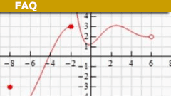
In a graph of a function, when we approach a particular value, we can do it either from the right side or from the left side of the graph. Mathematically, when we say that, ‘x tends to c’, it can mean either that x is infinitesimally larger than c or it is infinitesimally smaller than c’.

[tex]\lim{x \to c}f(x)[/tex]

Here, let:

[tex]x = c + h[/tex]

and

[tex]as~~x \to c~~;h \to 0[/tex]

As such, ‘x’ is infinitesimally larger than ‘x’. On a graph, ‘x’ lies on the right of x, and such such a limit is called the ‘Right Hand Limit'(RHL). Whereas, if we take, x = c – h, it is called the ‘Left Hand Limit'(LHL). It is denoted as follows:

[tex]RHL:~~~\lim_{x \to c^+} f(x)~~=~~\lim_{h \to 0} f(c + h)[/tex]

[tex]LHL:~~~\lim_{x \to c^-} f(x)~~=~~\lim_{h \to 0} f(c – h)[/tex]

For a continuous function, both these values are equal to each other and also to f(c).

4. List of standard limits

In addition to the identities given in the equation box below, the following standard limits are helpful in evaluating limits of compound functions. The following listed limits are commonly used and are hence enlisted for easy reference:

[tex]\lim_{x \to c} x = c[/tex]

[tex]\lim_{x \to 0} \frac{1}{x} = \infty[/tex]

[tex]\lim_{x \to \infty} x = \infty[/tex]

[tex]\lim_{x \to 0} \frac{\sin(x)}{x} = 1[/tex]

[tex]\lim_{x \to 0} \frac{\tan(x)}{x} = 1[/tex]

[tex]\lim_{x \to 0} \frac{1 – \cos(x)}{x} = 0[/tex]

[tex]\lim_{x \to a} \frac{x^n – a^n}{x – a} = na^{n – 1}[/tex]

[tex]\lim_{x \to a} \frac{\sin(x – a)}{x – a} = 1[/tex]

[tex]\lim_{x \to a} \frac{\tan(x – a)}{x – a} = 1[/tex]

[tex]\lim_{x \to 0} \frac{log_e(1 + x)}{x} = 1[/tex]

[tex]\lim_{x \to 0} \frac{a^x – 1}{x} = log_e a[/tex]

[tex]\lim_{x \to 0} \frac{e^x – 1}{x} = 1[/tex]

This has not to be confused with limits of sequences of functions as considered in functional analysis, e.g. example 5.9. in https://www.physicsforums.com/insights/hilbert-spaces-relatives/

Comment Thread