How to Visualize the 2-D Particle in a Box

Introduction

The particle in a box is a staple of entry-level Quantum Mechanics classes because it provides a meaningful contrast between classical and quantum dynamics. It is one of the few problems that can be solved exactly, without approximations. Despite this, I would wager that most of you solved only the 1-D particle in a box problem, and didn’t worry too much about the bigger picture, visualizing the solution, or higher-dimensional examples. Many other people reading this might be involved in a scientific discipline other than physics, but nevertheless might be interested in the peculiarities of Quantum Mechanics (QM).

In this Insight, I’ll briefly outline why the particle in a box problem is important, what the solutions mean, and what the solution to higher dimensional (2-D) boxes looks like. Along the way, you might even pick up some useful MATLAB code for creating your own visualizations.

Problems with Intuition

In the 1-D example, a particle is free to move (potential energy [itex]V = 0[/itex]) backward and forward along a straight line of length [itex]L_x[/itex]. No forces act on the particle when it is in the box. The walls of this 1-D “box” are considered to be impenetrable, as the space outside the box has an infinitely large potential energy ([itex]V = \infty[/itex]).

Let’s say that the box is 1 meter long. Classical mechanics says that the particle can move at any speed along the line, and it is equally likely to be found at any point along the line. Pretty straightforward, right?

Now, let’s say that the box is 1 nanometer long (1e-9m). On this scale, QM is applicable, rather than classical mechanics. The quantum mechanical solution (briefly outlined below) says the following:

1. The particle is more likely to be found in certain positions than others, depending on its energy.
2. There are “blind spots”, or places where the particle can never be detected.
3. The energy of the particle must obey a discrete set of energy levels.
4. The particle can not have zero energy, so it is always moving.

Needless to say, the QM solution stands in stark contrast to the simple and intuitive classical solution!

The Schrödinger Equation

To solve this problem with QM, the time-dependent Schrödinger equation is used. I’m going to omit many details in this discussion, as our primary focus is in understanding the basic problem. I encourage you to read the references for the full details.

[tex]i \hbar \frac{\partial}{\partial t} \Psi(x,t) = -\frac{\hbar^2}{2m} \frac{\partial^2}{\partial x^2} \Psi(x,t) + V(x)\Psi(x,t)[/tex]

The variables in this equation, if you aren’t familiar with them, are:

•  [itex]\Psi[/itex] is the wave function for the particle. The wave function is important as the position, energy, and momentum of the particle can all be obtained from it.
• [itex]V[/itex] is the potential energy of the particle.
• [itex]x[/itex] is the position of the particle.
• [itex]t[/itex] is time.
• [itex]\hbar[/itex] is the reduced Planck’s constant.
• [itex]m[/itex] is the mass of the particle.
• [itex]i[/itex] is the imaginary unit.

Since the potential energy [itex]V[/itex] is time-independent (it depends only on the position [itex]x[/itex]), we can perform a separation of variables by assuming that [itex]\Psi(x,t) = \psi(x) \phi(t)[/itex]. Substituting this into the above equation creates a situation where the left side depends only on time [itex]t[/itex], and the right side depends only on position [itex]x[/itex]. This can only be the case if both sides are equal to the same constant, which we call [itex]E[/itex].

[tex]-\frac{\hbar^2}{2m}\frac{\partial^2 \psi(x)}{\partial x^2} + V(x)\psi(x) = E\psi(x)[/tex]

[tex]i\hbar \frac{\partial \phi(t)}{\partial t} = E\phi(t)[/tex]

This means that the solutions to the position equation are time-independent, and for this reason, these solutions are called stationary states. The stationary states correspond to definite values of the energy.

The 1-D Wavefunction

After solving the time-dependent equation, you end up with two solutions: one that describes the position, and the other that describes the time dependence.

[tex]\psi(x) = A\sin(kx) + B\cos(kx)[/tex]

[tex]\phi(t) = e^{-i \omega t}[/tex]

But as we said before, the potential walls need to be impenetrable, so the boundary requirement is that [itex]\psi(0) = \psi(L_x) = 0[/itex]. This boundary requirement results in:

[tex]\psi(x) = A\sin(kx)[/tex]

where [itex]k[/itex] must be equal to [itex]n\pi/L_x[/itex] to satisfy [itex]\psi(L_x)=0[/itex]. The variable [itex]k[/itex] is called the wavenumber, as it is related to the total energy of the particle:

[tex]E_n = \hbar \omega = \frac{\hbar^2 k^2}{2m}[/tex]

Simulating the 1-D Solution

So the above solutions tell us everything. If [itex]n=3[/itex], for instance, then the energy of the particle is [itex]E_3[/itex], its momentum is [itex]p=\sqrt{2E_3m}[/itex], its position is described by [itex]\psi(x)[/itex], the time dependence is [itex]\phi(t)[/itex], and [itex]A = \sqrt{2/L_x}[/itex] is the normalization:

[tex]\Psi(x,t) = \psi(x) \phi(t) = \sqrt{\frac{2}{L_x}} \sin(kx) e^{-i \omega t}[/tex]

You can make a .gif movie of the time evolution in MATLAB as follows. Note that I assign a value of 1 to all of the constants for simplicity and plot only the real part of the function. Click the link to view the code, or click the image to view the animation.

View the code for the 1-D time-simulation

In particular, note the spots where the wave function is always zero. These are the places where the particle will never be found!

Simulating the 2-D Solution

In 2-D, the problem is similar except that the particle is confined to a box of width [itex]L_x[/itex] and height [itex]L_y[/itex]. Remember how we used separation of variables to solve the 1-D equation? Well, it turns out that after applying the same method once to the 2-D equation, you end up with:

[tex]-\frac{\hbar^2}{2m}\left( \frac{\partial^2 \psi(x,y)}{\partial x^2} + \frac{\partial^2 \psi(x,y)}{\partial y^2} \right) + V(x,y)\psi(x,y) = E\psi(x,y)[/tex]

[tex]i\hbar \frac{\partial \phi(t)}{\partial t} = E\phi(t)[/tex]

To continue the solution, you can actually use separation of variables again to separate the x and y components, [itex]\psi(x,y) = f(x)g(y)[/itex]. This leads to an equation very similar to the 1-D case (details here and here), so we know that [itex]f(x)[/itex] is just the solution to the 1-D model, and [itex]g(y)[/itex] has a similar form (note how the normalization changed):

[tex]\Psi(x,y,t) = \psi(x,y) \phi(t) = f(x) g(y) \phi(t) [/tex]

[tex] \Psi(x,y,t) =  \sqrt{\frac{4}{L_x L_y}} \sin(k_x x) \sin(k_y y) e^{-i \omega t}[/tex]

Armed with the 2-D expression, you can make some simple adjustments to the previous MATLAB code to view a time-simulation of the function.

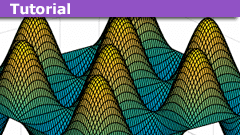
Here is the time-simulation for [itex](n_x,n_y) = (4,4)[/itex]. In this case, the spots where the wave function is always zero are more numerous and form a grid.

View the code for the 2-D time-simulation of (4,4)

In this last simulation I take it a step further and do the simulation for several combinations of  [itex](n_x,n_y)[/itex]:

View code for the full 2-D time-simulation

Feedback

Please leave comments or send me a message with any feedback so that I can improve future posts!

Learn More

1. http://galileo.phys.virginia.edu/classes/252/2d_wells.html
2. http://en.wikipedia.org/wiki/Particle_in_a_box
3. http://hyperphysics.phy-astr.gsu.edu/hbase/quantum/pbox.html
4. https://youtu.be/lGKKdLmRNQw
5. http://sm286.cyberbass.com/Lecture%20Notes/Supplimentry%20Notes/N05%20Particle%20in%20a%20Box%202D.pdf